Chapter 13 Element 6: Tidyverse – tidyr
13.1 Learning Objectives
Tidy data is defined as:
- One observation per row,
- One variable per column, and
- One observational unit per data frame.
| weight | group |
|---|---|
| 4.2 | ctrl |
| 5.6 | ctrl |
| 5.2 | ctrl |
| 6.1 | ctrl |
| 4.5 | ctrl |
| 4.6 | ctrl |
| trt2 | trt1 | ctrl |
|---|---|---|
| 6.3 | 4.8 | 4.2 |
| 5.1 | 4.2 | 5.6 |
| 5.5 | 4.4 | 5.2 |
| 5.5 | 3.6 | 6.1 |
| 5.4 | 5.9 | 4.5 |
| 5.3 | 3.8 | 4.6 |
| 4.9 | 6.0 | 5.2 |
| 6.2 | 4.9 | 4.5 |
| 5.8 | 4.3 | 5.3 |
| 5.3 | 4.7 | 5.1 |
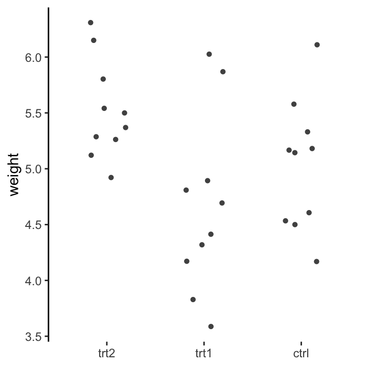
Data should be arranged in a format that makes downstream analysis easier, instead of forcing functions to work on poorly formatted data. We can see this with the PlantGrowth data set (table 13.1). The long, tidy format allows us to carry out easy commands like making plots, defining linear models and even calculating group-wise descriptive statistics. A more typical way to store this data would be like table 13.2. But this would make it much more difficult to work with. Can you imagine how to draw the same box plot if your data was in this format? It’s possible, but not nice!
Some statisticians, bioinformaticians and data scientists estimate that about three-quarters of their time is spent on “data munging”, that is, getting data cleaned-up and tidy so that they can actually analyse it.
library(tidyverse)
# PG_wide <- read_tsv("http://www.scavetta.academy/IDAwR/data/PlantGrowth_Wide.txt")
PG_wide <- read_tsv("data/PlantGrowth_Wide.txt")
glimpse(PG_wide)
# Rows: 10
# Columns: 3
# $ ctrl <dbl> 4.2, 5.6, 5.2, 6.1, 4.5, 4.6, 5.2, 4.5, 5.3, 5.1
# $ trt1 <dbl> 4.8, 4.2, 4.4, 3.6, 5.9, 3.8, 6.0, 4.9, 4.3, 4.7
# $ trt2 <dbl> 6.3, 5.1, 5.5, 5.5, 5.4, 5.3, 4.9, 6.2, 5.8, 5.3Notice that we used tidyr::read_tsv() instead of utils::read.delim(). These new functions from the tidyr package are a bit more convenient than the base package functions and all contain an _ instead of a ., which is a common feature in tidyverse syntax.
This has one key consequence here. The data frame is not just a data frame, but it’s also a tibble:
# [1] "spec_tbl_df" "tbl_df" "tbl" "data.frame"This has a couple consequence. First, when we print it to the screen, we’ll only get the first 10 lines by default, which makes it pretty convenient for prototyping functions and collections of functions.
# # A tibble: 10 x 3
#     ctrl  trt1  trt2
#    <dbl> <dbl> <dbl>
#  1  4.17  4.81  6.31
#  2  5.58  4.17  5.12
#  3  5.18  4.41  5.54
#  4  6.11  3.59  5.5
#  5  4.5   5.87  5.37
#  6  4.61  3.83  5.29
#  7  5.17  6.03  4.92
#  8  4.53  4.89  6.15
#  9  5.33  4.32  5.8
# 10  5.14  4.69  5.26
Here, that isn’t so important since we only have 10 lines, but in general the output format will be nicer and fit at many columns as can fit onto your screen, but we’ll also see the type of each column, which is pretty handy.
The other major consequence is that tibbles stay data frames no matter what. That means that:
# # A tibble: 10 x 1
#     trt2
#    <dbl>
#  1  6.31
#  2  5.12
#  3  5.54
#  4  5.5
#  5  5.37
#  6  5.29
#  7  4.92
#  8  6.15
#  9  5.8
# 10  5.26
is the same as
# # A tibble: 10 x 1
#     trt2
#    <dbl>
#  1  6.31
#  2  5.12
#  3  5.54
#  4  5.5
#  5  5.37
#  6  5.29
#  7  4.92
#  8  6.15
#  9  5.8
# 10  5.26
if we just had a regular data frame this wouldn’t be the case:
PG_wide_NOTIBBLE <- read.delim("http://www.scavetta.academy/IDAwR/data/PlantGrowth_Wide.txt")
PG_wide_NOTIBBLE[,3]
# [1] 6.3 5.1 5.5 5.5 5.4 5.3 4.9 6.2 5.8 5.3# trt2
# 1 6.3
# 2 5.1
# 3 5.5
# 4 5.5
# 5 5.4
# 6 5.3
# 7 4.9
# 8 6.2
# 9 5.8
# 10 5.3This is pretty consequential if you recognize that base R likes to switch between data frames and vectors – So be careful here!
Now that we have some small play data, let’s try to complete the following exercises using PG_wide:
| group | avg | stdev |
|---|---|---|
| trt2 | 5.5 | 0.44 |
| trt1 | 4.7 | 0.79 |
| ctrl | 5.0 | 0.58 |
| ctrl | trt1 | trt2 |
|---|---|---|
| -1.48 | 0.188 | 1.771 |
| 0.94 | -0.619 | -0.917 |
| 0.25 | -0.316 | 0.032 |
| 1.85 | -1.349 | -0.059 |
| -0.91 | 1.523 | -0.352 |
| -0.72 | -1.047 | -0.533 |
| 0.24 | 1.725 | -1.369 |
| -0.86 | 0.289 | 1.410 |
| 0.51 | -0.430 | 0.619 |
| 0.19 | 0.037 | -0.601 |
| Df | Sum Sq | Mean Sq | F value | Pr(>F) | |
|---|---|---|---|---|---|
| group | 2 | 3.8 | 1.88 | 4.8 | 0.02 |
| Residuals | 27 | 10.5 | 0.39 | NA | NA |
13.1 The pipe operator - %>%
Before we get into tidyverse functions, let’s cover a fundamental punctuation: %>%, aka the pipe operator. The pipe operator is a shorthand for calling functions, such that:
function(x) == x %>% function() (When speaking the commands say and then.)
This is not specific to dplyr functions. It can be used with any R functions:
# [1] 5.5# [1] 5.5The advantage here is that we can string together a long series of functions that would be very difficult to read in the regular R nomenclature, which we’ll see in a minute as our functions get more complex.
13.1 Tidy Data with the tidyr Package
To understand tidy data, we’ll consider a generic example with a data frame, PlayData (see figure ??).
# Create a new play dataset to work on:

PlayData <- read_tsv("data/PlayData.txt")

# PlayData <- data.frame(type = rep(c("A", "B"), each = 2),
#                        time = 1:2,
#                        height = seq(10, 40, 10),
#                        width = seq(50, 80, 10))
To work with our data in R, we want all variables in their own columns. To achieve this, we will gather our data into a long, tidy form. To understand what this means, we need to realize that there are essentially two different types of variables:
ID Variables are all the possible grouping variables which were measured. These include both independent and dependent categorical variables. ID variables are used to group, i.e. identify, our measurement variables. Our ID variables are type and time.
Measurement Variables are what was measured, here that’s the height and width.
13.1 Pivot to longer
Until recently the go-to function to get tidy data was tidyr::gather(). However, this has been supplanted by the much more flexible tidyr::pivot_longer(). This function takes four arguments:
- The wide data frame to make long (i.e. tidy).
- The ID (specified with
-) or MEASURE variables. - The name of the output column for the KEY.
- The name of the output column for the VALUE.
| type | time | key | value |
|---|---|---|---|
| A | 1 | height | 10 |
| A | 1 | width | 50 |
| A | 2 | height | 20 |
| A | 2 | width | 60 |
| B | 1 | height | 30 |
| B | 1 | width | 70 |
| B | 2 | height | 40 |
| B | 2 | width | 80 |
This will convert the remaining column headers into the 3rd ID variable, key, and produce the tidy data frame, shown above. HINT: If you want to select all columns in a data frame, i.e. all columns are MEASURE columns, you can use everything().
PG_wide, use the pivot_longer() to produce `PG_tidy
Now that you have long tidy data. Revisit the exercises from above:
Now that you have an idea about pivoting, let’s look at the other direction
13.1 Pivot to Wider
We can re-arrange our data and make it wider. e.g. to return to our original data frame, we can use:
| type | time | height | width |
|---|---|---|---|
| A | 1 | 10 | 50 |
| A | 2 | 20 | 60 |
| B | 1 | 30 | 70 |
| B | 2 | 40 | 80 |
Likewise, we can spread our data so that each category of time is now a separate variable.
| type | key | 1 | 2 |
|---|---|---|---|
| A | height | 10 | 20 |
| A | width | 50 | 60 |
| B | height | 30 | 40 |
| B | width | 70 | 80 |
Or so that type is defined in separate variables
| time | key | A | B |
|---|---|---|---|
| 1 | height | 10 | 30 |
| 1 | width | 50 | 70 |
| 2 | height | 20 | 40 |
| 2 | width | 60 | 80 |
The three transformation function scenarios are straight-forward, if our starting point is tidy data! But the power of tidy data becomes apparent when grouping our data according to a factor variable. This allows us to apply not only transformation functions, but aggregation functions as well. For this we turn to the dplyr package.