Chapter 12 2.1.5 Tidy data

12.1 Learning Objectives

It this chapter we’ll get into detail about what tidy means. Tidy data is defined as:

One observation per row,
One variable per column, and
One observational unit per data frame.

12.2 Example

Consider the following data frames:

Table 12.1: The long, tidy data frame.
weight	group
4.2	ctrl
5.6	ctrl
5.2	ctrl
6.1	ctrl
4.5	ctrl
4.6	ctrl

Table 12.2: A wide, messy data frame.
ctrl	trt1	trt2
4.2	4.8	6.3
5.6	4.2	5.1
5.2	4.4	5.5
6.1	3.6	5.5
4.5	5.9	5.4
4.6	3.8	5.3
5.2	6.0	4.9
4.5	4.9	6.2
5.3	4.3	5.8
5.1	4.7	5.3

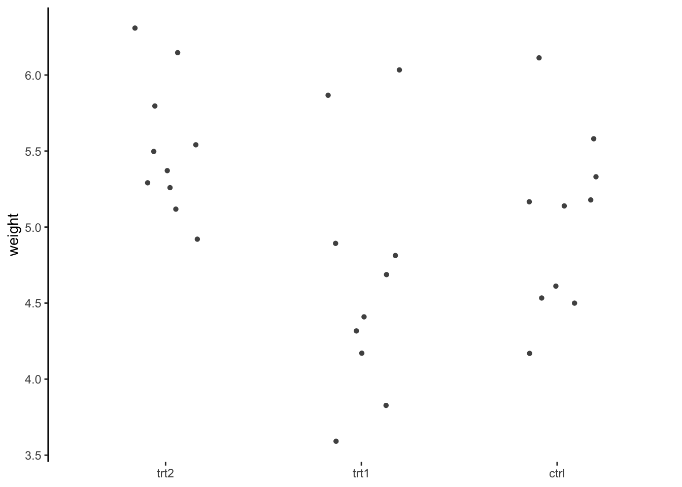
Data should be arranged in a format that makes downstream analysis easier, instead of forcing functions to work on poorly formatted data. We can see this with the PlantGrowth data set (table 12.1). The long, tidy format allows us to carry out easy commands like making plots, defining linear models and even calculating group-wise descriptive statistics. A more typical way to store this data would be like table 12.2. But this would make it much more difficult to work with. Can you imagine how to draw the same box plot if your data was in this format? It’s possible, but not nice!

Some statisticians, bioinformaticians and data scientists estimate that about three-quarters of their time is spent on “data munging,” that is, getting data cleaned-up and tidy so that they can actually analyse it.

Exercise 12.1 Create the wide format of the PlantGrowth data set using the commands given below

This will switch from long to wide format:

library(tidyverse)

PG_wide <- PlantGrowth %>% 
  mutate(id = rep(1:10,3)) %>% 
  pivot_wider(names_from = group, values_from = weight) %>% 
  select(-id)

glimpse(PG_wide)

## Rows: 10
## Columns: 3
## $ ctrl <dbl> 4.2, 5.6, 5.2, 6.1, 4.5, 4.6, 5.2, 4.5, 5.3, 5.1
## $ trt1 <dbl> 4.8, 4.2, 4.4, 3.6, 5.9, 3.8, 6.0, 4.9, 4.3, 4.7
## $ trt2 <dbl> 6.3, 5.1, 5.5, 5.5, 5.4, 5.3, 4.9, 6.2, 5.8, 5.3

Now that we have some messy data, let’s try to complete the following exercises using PG_wide:

Exercise 12.2 Draw a jittered dot plot of the weight described by each treatment type. We did this earlier in the course. The result should look like below. How would you go about doing this with PG_wide?

Exercise 12.3 Calculate the group-wise mean and standard deviation for all 10 observations in each treatment group using PG_wide instead of PlantGrowth. What functions would you use for this?

group	avg	stdev
trt2	5.5	0.44
trt1	4.7	0.79
ctrl	5.0	0.58

Exercise 12.4 Perform a z-score transformation within each treatment in the PG_wide data frame type using the scale() function. Your results should look like below.

ctrl	trt1	trt2
-1.48	0.188	1.771
0.94	-0.619	-0.917
0.25	-0.316	0.032
1.85	-1.349	-0.059
-0.91	1.523	-0.352
-0.72	-1.047	-0.533
0.24	1.725	-1.369
-0.86	0.289	1.410
0.51	-0.430	0.619
0.19	0.037	-0.601

Exercise 12.5 Calculate a 1-way ANOVA of each plant’s weight described by it’s treatment using the PG_wide data frame. Do you think this is easy in this case? The results we received previously look like:

Table 12.3: The results of a one-way ANOVA on the plant growth data set.
	Df	Sum Sq	Mean Sq	F value	Pr(>F)
group	2	3.8	1.88	4.8	0.02
Residuals	27	10.5	0.39	NA	NA

12.3 The pipe operator - %>%

We’ve seen all the great bits of the tidyverse in action already. Here, we’ll review some fundamentals. First, the punctuation: %>%, aka the forward-pipe operator. The forward-pipe operator is a shorthand for calling functions, such that:

function(x) == x %>% function() (When speaking the commands say and then.)

This is not specific to dplyr functions. It can be used with any R functions:

aa <- 1:10

# The usual way
mean(aa)

## [1] 5.5

# or with the pipe operator
aa %>% 
  mean()

## [1] 5.5

The advantage here is that we can string together a long series of functions that would be very difficult to read in the regular R nomenclature, which we’ll see in a minute as our functions get more complex.

12.4 Tidy Data with the `tidyr` Package

To understand tidy data, we’ll consider a generic example with a data frame, PlayData (see figure ??).

# Create a new play dataset to work on:
PlayData <- read_tsv("data/PlayData.txt")

To work with our data in R, we want all variables in their own columns. To achieve this, we will gather our data into a long, tidy form. To understand what this means, we need to realize that there are essentially two different types of variables:

ID Variables are all the possible grouping variables which were measured. These include both independent and dependent categorical variables. ID variables are used to group, i.e. identify, our measurement variables. Our ID variables are type and time.

Measurement Variables are what was measured, here that’s the height and width.

12.5 Pivot to longer

Until recently the go-to function to get tidy data was tidyr::gather(). However, this has been supplanted by the much more flexible tidyr::pivot_longer(). This function takes two arguments:

The wide data frame to make long (i.e. tidy).
The ID (specified with -) or MEASURE variables (simply named as such).

I usually also specify the:

The name of the output column for the KEY, using the names_to argument.
The name of the output column for the VALUE using the values_to argument.

PlayData %>% 
  pivot_longer(-c(type, time), names_to = "key", values_to = "value") -> PlayData_t

type	time	key	value
A	1	height	10
A	1	width	50
A	2	height	20
A	2	width	60
B	1	height	30
B	1	width	70
B	2	height	40
B	2	width	80

This will convert the remaining column headers into the 3rd ID variable, key, and produce the tidy data frame, shown above. HINT: If you want to select all columns in a data frame, i.e. all columns are MEASURE columns, you can use everything().

Exercise 12.6 Starting with PG_wide, use the pivot_longer() to produce `PG_tidy

PG_wide %>% 
  pivot_longer(cols = everything(), names_to = "weight", values_to = "group") -> PG_long

Now that you have long tidy data. Revisit the exercises from above for PG_wide. They are much easier using a tidy data version of the data frame!

Exercise 12.7 Using PlantGrowth, draw a jittered dot plot of the weight described by each treatment type.

Exercise 12.8 Using PlantGrowth, calculate the group-wise mean and standard deviation for all 10 observations in each treatment group.

Exercise 12.9 Using PlantGrowth, perform a z-score transformation within each treatment type.

Exercise 12.10 Using PlantGrowth, calculate a 1-way ANOVA of each plant’s weight described by it’s treatment.

Now that you have an idea about pivoting, let’s look at the other direction

12.6 Pivot to Wider

We can re-arrange our data and make it wider. e.g. to return to our original data frame, we can use:

PlayData_t %>%
  pivot_wider(names_from = "key", values_from = "value")

type	time	height	width
A	1	10	50
A	2	20	60
B	1	30	70
B	2	40	80

We saw this in the code above to get the PG_wide.

Likewise, we can pivot_wider so that each category of time is now a separate variable.

PlayData_t %>%
  pivot_wider(names_from = "time", values_from = "value")

type	key	1	2
A	height	10	20
A	width	50	60
B	height	30	40
B	width	70	80

Or so that type is defined in separate variables

PlayData_t %>%
  pivot_wider(names_from = "type", values_from = "value")

time	key	A	B
1	height	10	30
1	width	50	70
2	height	20	40
2	width	60	80

The three transformation function scenarios are straight-forward, if our starting point is tidy data! But the power of tidy data becomes apparent when grouping our data according to a factor variable. This allows us to apply not only transformation functions, but aggregation functions as well. For this we turn to the dplyr package.

ctrl	trt1	trt2
4.2	4.8	6.3
5.6	4.2	5.1
5.2	4.4	5.5
6.1	3.6	5.5
4.5	5.9	5.4
4.6	3.8	5.3
5.2	6.0	4.9
4.5	4.9	6.2
5.3	4.3	5.8
5.1	4.7	5.3

ctrl	trt1	trt2
4.2	4.8	6.3
5.6	4.2	5.1
5.2	4.4	5.5
6.1	3.6	5.5
4.5	5.9	5.4
4.6	3.8	5.3
5.2	6.0	4.9
4.5	4.9	6.2
5.3	4.3	5.8
5.1	4.7	5.3