9 Effects of Meditation Case Study
In this case study we’ll look at data simulated from a real-world, published experiment. We’ll explore some new key concepts in this chapter: rearranging data to make it easier to work with.
As an exercise in manipulating data, consider the meditation data-set. This data-set contains the expression values of 6 pro-inflammatory genes. These are results from a published study. The researchers wanted to test if these genes are deferentially expressed after meditation in people who regularly meditate, compared to non-meditating control individuals. Expression levels were measured in the morning (time 1) and after (time 2) a full day of meditation, by experienced meditators, or leisure, by the control group.
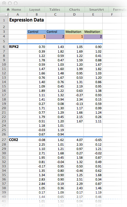
Figure 9.1: The medi data-set as it would be typically stored as an Excel spreadsheet. Although this is human-readable, it is not an efficient way of storing data!
Exercise 9.1 (Messy versus Tidy) What is the problem with the data format in figure 9.1?
Figure 9.1 is an example of a typical Excel spreadsheet. Here, column headers are found in the middle of the spread sheet and the results for each measured gene is contained in its own table on the same worksheet. In addition, column headers are colour-coded and there is plenty of white space for formatting purposes.
As a first step towards tidy data, we will remove all white space, colour-coding and floating labels. The data-set in Figure 9.2 resembles the long list file we have already encountered. It’s not perfect, but it’s a good start.
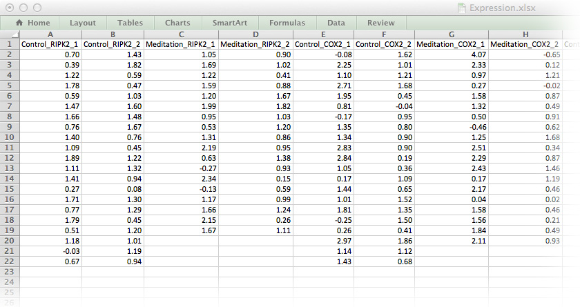
Figure 9.2: The medi data-set in a format ready for importing into R.
9.1 Tidy data
Reshaping and tidying our data (Tidy Data Paper)[http://vita.had.co.nz/papers/tidy-data.pdf]
- Each row is an observation
- Each column is a variable
- Each type of observational unit forms a table
df = pd.DataFrame({
            'name': ["John Smith", "Jane Doe", "Mary Johnson"],
            'treatment_a': [None, 16, 3],
            'treatment_b': [2, 11, 1]})
print(df)
#>            name  treatment_a  treatment_b
#> 0    John Smith          NaN            2
#> 1      Jane Doe         16.0           11
#> 2  Mary Johnson          3.0            1
df_melt = pd.melt(df, id_vars='name')
print(df_melt)
#>            name     variable  value
#> 0    John Smith  treatment_a    NaN
#> 1      Jane Doe  treatment_a   16.0
#> 2  Mary Johnson  treatment_a    3.0
#> 3    John Smith  treatment_b    2.0
#> 4      Jane Doe  treatment_b   11.0
#> 5  Mary Johnson  treatment_b    1.0
Tidy pivot_table
df_melt_pivot = pd.pivot_table(df_melt,
                               index='name',
                               columns='variable',
                               values='value')

print(df_melt_pivot)
#> variable      treatment_a  treatment_b
#> name
#> Jane Doe             16.0         11.0
#> John Smith            NaN          2.0
#> Mary Johnson          3.0          1.0
This results in a hierarchical index, so to get a regular flat data frame, call
df_melt_pivot.reset_index()
#> variable          name  treatment_a  treatment_b
#> 0             Jane Doe         16.0         11.0
#> 1           John Smith          NaN          2.0
#> 2         Mary Johnson          3.0          1.0
print(df_melt_pivot)
#> variable      treatment_a  treatment_b
#> name
#> Jane Doe             16.0         11.0
#> John Smith            NaN          2.0
#> Mary Johnson          3.0          1.0
9.2 groupby operations
- groupby: split-apply-combine
- split data into separate partitions
- apply a function on each partition
- combine the results
print(df_melt)
#>            name     variable  value
#> 0    John Smith  treatment_a    NaN
#> 1      Jane Doe  treatment_a   16.0
#> 2  Mary Johnson  treatment_a    3.0
#> 3    John Smith  treatment_b    2.0
#> 4      Jane Doe  treatment_b   11.0
#> 5  Mary Johnson  treatment_b    1.0
df_melt.groupby('name')['value'].mean()
#> name
#> Jane Doe        13.5
#> John Smith       2.0
#> Mary Johnson     2.0
#> Name: value, dtype: float64
Exercise 9.2 (Import data) Import Expression.txt. Save it as an object called medi.
Exercise 9.3 (Tidy data) Convert the data set to a tidy format.
Exercise 9.4 (Calculate Statistics) Calculate each of the following statistics for each of the unique 24 combinations of gene, treatment and time:
-
averagethe mean of the value -
nthe number of observations in each group -
SEMThe standard error of the mean -
CIerrorThe 95% CI error defined by the t distribution -
lower95The upper 95% CI limit -
upper95The upper 95% CI limit
Exercise 9.5 (Export data) Now that you’ve processed your data, refer to the following table and save a file on your computer that contains the summary statistics.