Chapter 6 Objects
6.1 Take-home Messages
In R, everything that exists is an object:
- There are four common user-defined atomic vector types you’ll encounter in R.
- Vectors are 1-dimensional collections of 0 or more elements of a common data type.
- Data frames are 2-dimensional collections of 0 or more vectors.
- The class of an object dictates how it will be handled by different functions.
Objects are anything which14 can be assigned a name. They can refer to a wide variety of different data types, including constants, various data structures, functions or graphs.15 Work in R is centered around objects and their classes, and as such is referred to as an object-oriented language.16
R can store data in a variety of formats. In this workshop we will focus on the two most commonly used structures: vectors and data frames. However, as your R programming skills develop, you will likely encounter lists, matrices and arrays. These are described later in the chapter but will not be dealt with in class. The differences between the main data structures in R can be summarised as:17
| Name | Composition | Dimensions |
|---|---|---|
| Vector | Homogeneous | 1 |
| Matrix | Homogeneous | 2 |
| Array | Homogeneous | n |
| List | Heterogeneous | 1 |
| Data frame | Heterogeneous | 2 |
In addition to these 5 data structures, we’ll explore some fundamental properties of objects, such as type, attributes, and class, which will help you understand how R deals with objects later on.
6.2 Homogeneous Data-types
6.2.1 Vectors
Vectors are one-dimensional groups of individual data values. We have already encountered vectors on page ?? when we defined foo1 and foo2. Remember that these objects only contain the numerical series that we generated with the seq() function:
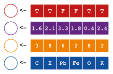
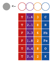
foo1## [1] 1 8 15 22 29 36 43 50 57 64 71 78 85 92 99foo2## [1] 1 7 13 19 25 31An important property of vectors, is that they can only contain one data type, thus they are homogeneous. There are many different data types in R. There are 6 user-defined atomic vector types.18 The four most common are:
| Typ | Description |
|---|---|
Logical |
TRUE/T/1 or FALSE/F/0 |
Integer |
Whole numbers |
Double |
Numeric (i.e. real numbers, including fractions) |
Character |
Words |
The numeric class refers to either double or integer. To find out the type of a vector, we can use the typeof() function.
typeof(foo2)## [1] "double"You may wonder why the type of foo2 is double (aka numeric) and not integer. This is due to how R predicted the type of data. If we want to force these values to be logical we’d have to use the special integer signifier L:
foo1 <- seq(1L, 100L, 7L)
typeof(foo1)
## [1] "integer"For the most part this will not make a difference in your work, but you may encounter problems when doing math on type double due to floating point errors, discussed on page 7.7. For our purposes, we are not bothered if an integer is stored as a double.
We can use c() to create vectors of other data types:
foo3 <- c("Liver", "Brain", "Testes", "Muscle",
"Intestine", "Heart")
typeof(foo3)
## [1] "character"foo4 <- c(TRUE, FALSE, FALSE, TRUE, TRUE, FALSE)
typeof(foo4)## [1] "logical"6.2.1.1 Atomic vector type hierarchy and coercion
When we assign a vector to an object, R automatically determines the atomic vector type.20 The atomic vector types have a hierarchical organisation according to increasing complexity: logical < integer < double < character. This kind of makes sense since logical can only be 0 or 1, and character can be everything. This means that R defaults to the highest level in the hierarchy.
test <- c(1:10, "bob")
test
## [1] "1" "2" "3" "4" "5" "6" "7" "8" "9" "10" "bob"typeof(test)## [1] "character"Since test is a character vector, I can’t do math on it!
mean(test)## Warning in mean.default(test): argument is not numeric or logical: returning NA## [1] NAA family of coercion functions are used to coerce one type to another.
as.numeric(test)## Warning: NAs introduced by coercion## [1] 1 2 3 4 5 6 7 8 9 10 NAEverything that looked like a number is converted to a number, but the contaminating character is replaced by an NA. Now I can do math, but I need to accommodate for the missing values.21
mean(as.numeric(test), na.rm = T)## Warning in mean(as.numeric(test), na.rm = T): NAs introduced by coercion## [1] 5.5We can determine the atomic vector type of an object by using typeof(), but sometimes we want to ask specifically if an object is of a specific type, in particular when we shift from interactive programming to scripting and writing our own functions.22 For this purpose there is a long list of is. functions that all return a logical vector.
is.numeric(foo1)## [1] TRUEis.integer(foo2)## [1] FALSEis.character(foo3)## [1] TRUEis.logical(foo4)## [1] TRUE6.2.2 Matrices
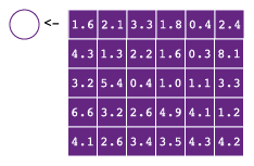
A matrix is a 2-dimensional vector, which means every element needs to be the same type. Matrices are incredibly convenient if you have a 2-dimensional grid of numbers on which you want to apply a mathmatical function, like linear algebra. To understand how matrices work, it’s useful to get familiar with attributes.
6.2.2.1 Setting object attributes
Almost all objects in R23 can have attributes, which can be accessed in a variety of ways. Table 6.2 lists the most typical attributes.
| Description | Attribute name | Accessor functions |
|---|---|---|
| Class | class |
class() |
| Column names | names |
names() |
| Dimensions | dim |
dim() |
| Row names | row.names |
row.names() |
| Dimension names | dimnames |
dimnames() |
| Commentary | comment |
comment() |
Matrices (and arrays, see below.) are just vectors with a dim attribute. Attributes can be obtained using attributes() and set in two ways. First, using attr(x, name), where x in an object and name is, typically, one of the attribute names in table 6.2.
aa <- foo1
attributes(aa)
## NULLaa## [1] 1 8 15 22 29 36 43 50 57 64 71 78 85 92 99attr(aa, "dim") <- c(3,5)
aa## [,1] [,2] [,3] [,4] [,5]
## [1,] 1 22 43 64 85
## [2,] 8 29 50 71 92
## [3,] 15 36 57 78 99attributes(aa)## $dim
## [1] 3 5# Remove attributes:
attributes(aa) <- NULL
aa## [1] 1 8 15 22 29 36 43 50 57 64 71 78 85 92 99However, name can be anything you want, so you are free to make your own attributes.
attr(aa, "owner") <- "Rick"
attributes(aa)
## $owner
## [1] "Rick"attributes(aa)$owner## [1] "Rick"Second, and more typical, is to default to the special accessor functions when they are available.
# Use the special accessor functions if available
dim(aa) <- c(3,5)
aa
## [,1] [,2] [,3] [,4] [,5]
## [1,] 1 22 43 64 85
## [2,] 8 29 50 71 92
## [3,] 15 36 57 78 99
## attr(,"owner")
## [1] "Rick"In the case of matrices, we have yet another method, matrix(), which gives us more control, e.g. filling row-wise, instead of the default column-wise.
attributes(aa) <- NULL
aa
## [1] 1 8 15 22 29 36 43 50 57 64 71 78 85 92 99aa <- matrix(aa, nrow = 3, byrow = TRUE)
aa## [,1] [,2] [,3] [,4] [,5]
## [1,] 1 8 15 22 29
## [2,] 36 43 50 57 64
## [3,] 71 78 85 92 99There are a some very convenient24 functions for working with columns and rows:{#matrices}
colMeans(aa)## [1] 36 43 50 57 64colSums(aa)## [1] 108 129 150 171 192rowMeans(aa)## [1] 15 50 85rowMeans(aa)## [1] 15 50 856.2.2.2 Matrix algebra
If you use the * operator to multiply two vectors – which we can now understand as 1 x n matrices – R will implement its particular type of vector recycling. If you want to do true matrix algebra, you’ll have to use the \%*\% operator for inner multiplication or the \%o\% operator for outer multiplication.
aa <- 1:6

# Inner multiplication
aa %*% aa # i.e. sum(aa * aa)
## [,1]
## [1,] 91# Outer multiplication
bb <- c(10, 20)
aa %o% bb## [,1] [,2]
## [1,] 10 20
## [2,] 20 40
## [3,] 30 60
## [4,] 40 80
## [5,] 50 100
## [6,] 60 1206.2.3 Arrays
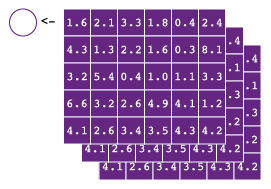
Arrays are n-dimensional vectors, which is to say a stack of n matrices.25 Just like matrices, they have to be all of the same type. Arrays are useful if you are working on longitudinal data but are not very convenient to work with. You are more likely to arrange your data into a data frame. A useful example is when working with images, the R (red), G (green), and B (blue) channels may be stored in a separate matrix, which together are stored as a multi-dimensional array (MDA). We can create arrays like matrices, changing the dimensions of a vector, or using the array() function for more control. Note that when we index arrays, there are three dimensions.
aa <- c(11:14, 21:24, 31:34)
dim(aa) = c(2, 2, 3)
aa
## , , 1
##
## [,1] [,2]
## [1,] 11 13
## [2,] 12 14
##
## , , 2
##
## [,1] [,2]
## [1,] 21 23
## [2,] 22 24
##
## , , 3
##
## [,1] [,2]
## [1,] 31 33
## [2,] 32 34ar <- array(c(11:14, 21:24, 31:34),
dim = c(2, 2, 3))
ar## , , 1
##
## [,1] [,2]
## [1,] 11 13
## [2,] 12 14
##
## , , 2
##
## [,1] [,2]
## [1,] 21 23
## [2,] 22 24
##
## , , 3
##
## [,1] [,2]
## [1,] 31 33
## [2,] 32 346.3 Heterogeneous Data-types
6.3.1 Lists
After 1-dimensional vectors, a 1-dimensional list is the most basic type of data structure in R. It’s basically a heterogeneous vector – where each element can be a different type. You may sometimes manually store data in a list, but because they can be a bit cumbersome to work with, you should have a good reason for doing so. For example, since they are a convenient way of storing heterogeneous data, many functions provide their results as a list.26 Actually, we’ve seen exactly that scenario already.
Plant_lm <- lm( weight ~ group, data=PlantGrowth)
typeof(Plant_lm)
## [1] "list"Plant_._lm is a list, and it has two attributes:
attributes(Plant_lm)## $names
##  [1] "coefficients"  "residuals"     "effects"       "rank"
##  [5] "fitted.values" "assign"        "qr"            "df.residual"
##  [9] "contrasts"     "xlevels"       "call"          "terms"
## [13] "model"
##
## $class
## [1] "lm"Which should be accessed with the appropriate accessor functions
names(Plant_lm)## [1] "coefficients" "residuals" "effects" "rank"
## [5] "fitted.values" "assign" "qr" "df.residual"
## [9] "contrasts" "xlevels" "call" "terms"
## [13] "model"class(Plant_lm)## [1] "lm"Remember, anything that is named can be accessed via the $ notation.
Plant.lm$coefficients## (Intercept) grouptrt1 grouptrt2
## 5.03 -0.37 0.49We can see a similar phenomenon with the ANOVA table, stored in Plant_anova.
Plant_anova <- anova(Plant_lm)
typeof(Plant_anova)
## [1] "list"# here there are four attributes:
attributes(Plant_anova)## $names
## [1] "Df" "Sum Sq" "Mean Sq" "F value" "Pr(>F)"
##
## $row.names
## [1] "group" "Residuals"
##
## $class
## [1] "anova" "data.frame"
##
## $heading
## [1] "Analysis of Variance Table\n" "Response: weight"class(Plant_anova)## [1] "anova" "data.frame"Here the two objects are both list types, but their classes are different.27 A class is simply an attribute that tells R what to do with this object. For example we can see that when we call print
print(Plant_lm) # identical to calling Plant_lm##
## Call:
## lm(formula = weight ~ group, data = PlantGrowth)
##
## Coefficients:
## (Intercept) grouptrt1 grouptrt2
## 5.032 -0.371 0.494summary(Plant_lm)##
## Call:
## lm(formula = weight ~ group, data = PlantGrowth)
##
## Residuals:
## Min 1Q Median 3Q Max
## -1.071 -0.418 -0.006 0.263 1.369
##
## Coefficients:
## Estimate Std. Error t value Pr(>|t|)
## (Intercept) 5.032 0.197 25.53 <2e-16 ***
## grouptrt1 -0.371 0.279 -1.33 0.194
## grouptrt2 0.494 0.279 1.77 0.088 .
## ---
## Signif. codes: 0 '***' 0.001 '**' 0.01 '*' 0.05 '.' 0.1 ' ' 1
##
## Residual standard error: 0.62 on 27 degrees of freedom
## Multiple R-squared: 0.264, Adjusted R-squared: 0.21
## F-statistic: 4.85 on 2 and 27 DF, p-value: 0.0159print(Plant_anova) # identical to calling Plant_anova## Analysis of Variance Table
##
## Response: weight
## Df Sum Sq Mean Sq F value Pr(>F)
## group 2 3.77 1.883 4.85 0.016 *
## Residuals 27 10.49 0.389
## ---
## Signif. codes: 0 '***' 0.001 '**' 0.01 '*' 0.05 '.' 0.1 ' ' 1summary(Plant_anova)## Df Sum Sq Mean Sq F value Pr(>F)
## Min. : 2.0 Min. : 3.8 Min. :0.39 Min. :4.8 Min. :0.02
## 1st Qu.: 8.2 1st Qu.: 5.4 1st Qu.:0.76 1st Qu.:4.8 1st Qu.:0.02
## Median :14.5 Median : 7.1 Median :1.14 Median :4.8 Median :0.02
## Mean :14.5 Mean : 7.1 Mean :1.14 Mean :4.8 Mean :0.02
## 3rd Qu.:20.8 3rd Qu.: 8.8 3rd Qu.:1.51 3rd Qu.:4.8 3rd Qu.:0.02
## Max. :27.0 Max. :10.5 Max. :1.88 Max. :4.8 Max. :0.02
## NA's :1 NA's :128This is a major feature of object-oriented programming (OOP) – functions behave differently given the class of an object.
We can make a list from scratch using list():
# create a list with 2 elements
l <- list(a = foo1, b = foo2)
l
## $a
## [1] 1 8 15 22 29 36 43 50 57 64 71 78 85 92 99
##
## $b
## [1] 1 7 13 19 25 316.3.2 Data Frames
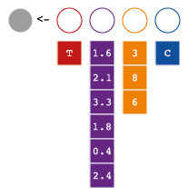
A data frame is a special type of list, where every every element is a vector of the same length. This means that data frames are two-dimensional tables, like you find in Excel.
Variables are vectors stored in vertical columns. Each variable can be it’s own data type (see table 6.1).
Observations are stored in horizontal rows.
This simple description leaves much room for interpretation. How you organize information in a data frame is important since it can influence how easily you can carry out downstream calculations. A very popular way to organize data frames is called tidy data, whereby data frames have:
- One observation per row,
- One variable per column, and are composed of
- One observational unit.
We will discus the best methods for formatting data in the section on tidy data.
Regardless of how you organize information in a data frame, there are two note-worthy aspects of data frames:
- Each column must be the same length.
- All data within a column must be of the same type.
This makes a lot of sense, since a data frame is just a list of vectors. You can see this in action by using tibble() to make a data frame (tibble variant) from the vectors foo2, foo3 and foo4.
foo_df <- tibble(foo4,foo3,foo2)
foo_df
## # A tibble: 6 × 3
## foo4 foo3 foo2
## <lgl> <chr> <dbl>
## 1 TRUE Liver 1
## 2 FALSE Brain 7
## 3 FALSE Testes 13
## 4 TRUE Muscle 19
## 5 TRUE Intestine 25
## 6 FALSE Heart 31typeof(foo_df)## [1] "list"The following table lists some of the most commonly used functions for working with data frames:
| Function | Description |
|---|---|
data.frame() |
Create a data frame. |
tibble() |
From the {tibble} package. Create a tibble variant of a data frame |
str() |
Structure of a data frame. |
glimpse() |
From the {dplyr} package. Structure of a data frame in a nicer format |
summary() |
Calculate summary statistics on each variable depending on its type |
dim() |
An accessor function for the Dimensions (number of rows and columns). |
names() |
An accessor function for the (column) names attribute. |
row.names() |
An accessor function for the row names. |
nrow() |
Number of rows |
ncol() |
Number of columns |
cbind() |
Add two data frames together by columns |
rbind() |
Add two data frames together by rows |
subset() |
Extract a subset of records, outdates but still in popular use. See the chapter on indexing and the filter() |
head() |
Show the head (first x number of rows) of the data frame |
tail() |
Show the tail (last x number of rows) of the data frame |
Let’s consider the foo_df data frame further. There are 3 attributes associated with this data frame (see table 6.2).
attributes(foo_df)## $names
## [1] "foo4" "foo3" "foo2"
##
## $row.names
## [1] 1 2 3 4 5 6
##
## $class
## [1] "tbl_df" "tbl" "data.frame"Which we can access by these common accessor functions:
# What are the column names?
names(foo_df)
## [1] "foo4" "foo3" "foo2"# What are the row names?
row.names(foo_df)## [1] "1" "2" "3" "4" "5" "6"# The class
class(foo_df)## [1] "tbl_df" "tbl" "data.frame"There are 6 rows (observations) and 3 columns (variables).
Take special note of the following unique featues of working with data frames:
- Variable names of a data frame (i.e. column headers) are themselves a character vector.
- To access specific columns by name, use
$notation to specify the name of the column, e.g.\$healthy. We already saw this with thePlantGrowthdata frame. - To select only those rows of interest, use the
subset()function and specify the data frame and the logical test of interest corresponding to specific criteria. We’ll get into more detail on what that all means in the next section. For now, just be aware that although you will seesubset()used, it has largely been supplanted byfilter()from the{dplyr}package.
Since the column names are just a character vector stored as an attribute, we can modify them independently of the data in the data frame.
names(foo_df)## [1] "foo4" "foo3" "foo2"# Reassign column names.
names(foo_df) <- myNames
names(foo_df)## [1] "healthy" "tissue" "quantity"# Select a single column by name.
foo_df$healthy## [1] TRUE FALSE FALSE TRUE TRUE FALSE# How many rows and columns does foo_df have?
dim(foo_df)## [1] 6 3It’s always useful to run these two functions on a data frame:
# str(foo_df) # base package, or
glimpse(foo_df) # Tidyverse, and
## Rows: 6
## Columns: 3
## $ healthy <lgl> TRUE, FALSE, FALSE, TRUE, TRUE, FALSE
## $ tissue <chr> "Liver", "Brain", "Testes", "Muscle", "Intestine", "Heart"
## $ quantity <dbl> 1, 7, 13, 19, 25, 31summary(foo_df)## healthy tissue quantity
## Mode :logical Length:6 Min. : 1.0
## FALSE:3 Class :character 1st Qu.: 8.5
## TRUE :3 Mode :character Median :16.0
## Mean :16.0
## 3rd Qu.:23.5
## Max. :31.06.3.2.1 stringsAsFactors
R version 4.0, released (April, 2020), changed the default value of the data.frame() argument stringsAsFactors to FALSE. Thus, if you have run this code on an older version of R what you actually see is this:
pre4_foo_df <- data.frame(foo4,foo3,foo2, stringsAsFactors = TRUE)
names(pre4_foo_df) <- myNames
glimpse(pre4_foo_df)
## Rows: 6
## Columns: 3
## $ healthy <lgl> TRUE, FALSE, FALSE, TRUE, TRUE, FALSE
## $ tissue <fct> Liver, Brain, Testes, Muscle, Intestine, Heart
## $ quantity <dbl> 1, 7, 13, 19, 25, 31We’ll discuss factors in ??. For what we’ll be doing, it does not make a difference.
6.4 Merging Data Frames
Merging two data frames according to a common variable is a typical command in data analysis. There are many varieties of merge and redundancy between functions. This guide presents functions in four packages:
basepackage functions will likely meet all your regular needsdplyr– If you’re using adplyrworkflow, see ??, default to these functions29.
Beginning with two data frames:
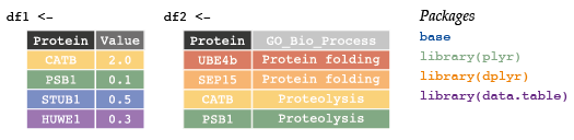
df1 <- data.frame(Protein = c("CATB", "PSB1", "STUB1", "HUWE1"),
                  Value = c(2.0, 0.1, 0.5, 0.3))
df2 <- data.frame(Protein = c("UBE4b", "SEP15", "CATB", "PSB1"),
                  GO = c(rep("Protein Folding", 2), rep("Proteolysis", 2)))
Use merge functions (and optional parameters) from either base package or dplyr to complete the following exercises.
6.4.1 Inner join
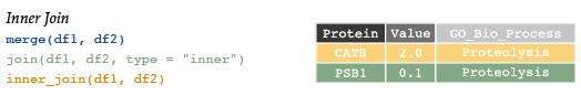
# Inner join:
merge(df1, df2)
## Protein Value GO
## 1 CATB 2.0 Proteolysis
## 2 PSB1 0.1 Proteolysislibrary(dplyr)
#inner
inner_join(df1, df2) # return all rows from x where there are matching values in y, and all columns from x and y## Joining, by = "Protein"## Protein Value GO
## 1 CATB 2.0 Proteolysis
## 2 PSB1 0.1 ProteolysisR automatically joins the frames by common variable names. To specify only the variables of interest, use merge(df1, df2, by = "Protein"). Additionally, use the by.x and by.y parameters if the matching variables have different names in the two data frames.
6.4.2 Outer join
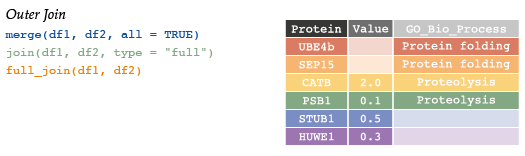
# Outer join:
merge(x = df1, y = df2, all = TRUE)
## Protein Value GO
## 1 CATB 2.0 Proteolysis
## 2 HUWE1 0.3 <NA>
## 3 PSB1 0.1 Proteolysis
## 4 SEP15 NA Protein Folding
## 5 STUB1 0.5 <NA>
## 6 UBE4b NA Protein Folding# join(df1, df2, type = "full") # return all rows from x, and all columns from x and y
full_join(df1, df2)## Joining, by = "Protein"## Protein Value GO
## 1 CATB 2.0 Proteolysis
## 2 PSB1 0.1 Proteolysis
## 3 STUB1 0.5 <NA>
## 4 HUWE1 0.3 <NA>
## 5 UBE4b NA Protein Folding
## 6 SEP15 NA Protein Folding6.4.3 Left join
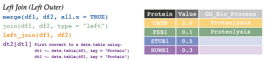
# Left outer:
merge(x = df1, y = df2, by = "Protein", all.x = TRUE)
## Protein Value GO
## 1 CATB 2.0 Proteolysis
## 2 HUWE1 0.3 <NA>
## 3 PSB1 0.1 Proteolysis
## 4 STUB1 0.5 <NA>#left outer
left_join(df1, df2) # return all rows from x, and all columns from x and y## Joining, by = "Protein"## Protein Value GO
## 1 CATB 2.0 Proteolysis
## 2 PSB1 0.1 Proteolysis
## 3 STUB1 0.5 <NA>
## 4 HUWE1 0.3 <NA>6.4.4 Right join
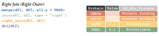
# Right outer:
merge(x = df1, y = df2, by = "Protein", all.y = TRUE)
## Protein Value GO
## 1 CATB 2.0 Proteolysis
## 2 PSB1 0.1 Proteolysis
## 3 SEP15 NA Protein Folding
## 4 UBE4b NA Protein Folding# #right outer (just reverse argument order)
# left_join(df2, df1)
#right join
right_join(df1, df2) # return all rows from x, and all columns from x and y## Joining, by = "Protein"## Protein Value GO
## 1 CATB 2.0 Proteolysis
## 2 PSB1 0.1 Proteolysis
## 3 UBE4b NA Protein Folding
## 4 SEP15 NA Protein Folding6.4.5 Anti-join & Semi-join
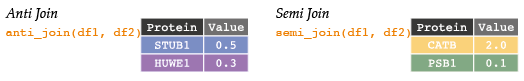
library(dplyr)
semi_join(df1, df2)
## Joining, by = "Protein"## Protein Value
## 1 CATB 2.0
## 2 PSB1 0.1anti_join(df1, df2)## Joining, by = "Protein"## Protein Value
## 1 STUB1 0.5
## 2 HUWE1 0.36.5 Ordering functions
There are a couple different ways to think about sorting data. Don’t confuse the following functions:
| Function | Description |
|---|---|
arrange() |
Part of the tidyverse. Rearranges a data frame according to a variable. |
sort() |
Returns a sorted vector (ascending or descending). Calls order() under-the-hood. |
order() |
Returns an index (integer vector) of the position of the ordered values (ascending or descending). Use this for data frames. Allows ordering on multiple vectors. |
rank() |
Returns the ranks of values in a vector, e.g. in non-parametric tests. |
foo_df## # A tibble: 6 × 3
## healthy tissue quantity
## <lgl> <chr> <dbl>
## 1 TRUE Liver 1
## 2 FALSE Brain 7
## 3 FALSE Testes 13
## 4 TRUE Muscle 19
## 5 TRUE Intestine 25
## 6 FALSE Heart 31foo_df %>%
arrange(tissue)## # A tibble: 6 × 3
## healthy tissue quantity
## <lgl> <chr> <dbl>
## 1 FALSE Brain 7
## 2 FALSE Heart 31
## 3 TRUE Intestine 25
## 4 TRUE Liver 1
## 5 TRUE Muscle 19
## 6 FALSE Testes 13foo_df %>%
arrange(desc(tissue))## # A tibble: 6 × 3
## healthy tissue quantity
## <lgl> <chr> <dbl>
## 1 FALSE Testes 13
## 2 TRUE Muscle 19
## 3 TRUE Liver 1
## 4 TRUE Intestine 25
## 5 FALSE Heart 31
## 6 FALSE Brain 7# A vector (or a variable in a data frame):
foo3## [1] "Liver" "Brain" "Testes" "Muscle" "Intestine" "Heart"sort(foo3) # values after ordering## [1] "Brain" "Heart" "Intestine" "Liver" "Muscle" "Testes"order(foo3) # index position after ordering## [1] 2 6 5 1 4 3foo3[order(foo3)] # i.e. sort()## [1] "Brain" "Heart" "Intestine" "Liver" "Muscle" "Testes"A cross join results in all combinations of all variables.
merge(x = df1, y = df2, by = NULL)## Protein.x Value Protein.y GO
## 1 CATB 2.0 UBE4b Protein Folding
## 2 PSB1 0.1 UBE4b Protein Folding
## 3 STUB1 0.5 UBE4b Protein Folding
## 4 HUWE1 0.3 UBE4b Protein Folding
## 5 CATB 2.0 SEP15 Protein Folding
## 6 PSB1 0.1 SEP15 Protein Folding
## 7 STUB1 0.5 SEP15 Protein Folding
## 8 HUWE1 0.3 SEP15 Protein Folding
## 9 CATB 2.0 CATB Proteolysis
## 10 PSB1 0.1 CATB Proteolysis
## 11 STUB1 0.5 CATB Proteolysis
## 12 HUWE1 0.3 CATB Proteolysis
## 13 CATB 2.0 PSB1 Proteolysis
## 14 PSB1 0.1 PSB1 Proteolysis
## 15 STUB1 0.5 PSB1 Proteolysis
## 16 HUWE1 0.3 PSB1 ProteolysisIn R, objects are synonymous with variables of other programming languages.↩︎
Objects are like files on your computer: They contain a wide variety of different data structures, can be modified, and their name may not relate to their contents. However, the extension of a file, like the class of an object, tells us about how we should handle this file. e.g. Which program will open it?↩︎
Object names can contain letters, numbers,
.or_, as long as it starts with a letter, or.followed by a letter. Note that object names are case sensitive.↩︎Although lists, matrices and arrays are presented here, it is worthwhile to return to this section after we have completed the workshop and explored working with data frame in depth, including indexing and Split-Apply-Combine. At that point you should be able to better understand how these data structures are handled in R.↩︎
The remaining two,
complexandraware unlikely to be encountered by beginners and we will not discuss them.↩︎Notice that R automatically assigns a type to each vector. A vector’s type determines what can be done with the data. Wrongly classified vectors are one of the most common causes of problems when programming in R!↩︎
Recall that we can influence this, as we saw above, using
Lto force anintegertype.↩︎Note that we can’t coerce a character to a logical vector, but if we did only have 0s and 1s, we could.↩︎
You’ll notice in the auto-complete that there are many
is.functions, which can test for more than use atomic vector types. In the examples here, the output length is always 1, since we are just testing for the type of an object, but that is not always the case. e.g. seeis.na()on page ??.↩︎The exception is the
NULLtype object.↩︎We typically use them on matrices since every value will be numeric or integer, but they also work on data frames.↩︎
Sometimes you’ll see arrays referred to as Multi-dimensional Arrays.↩︎
In some cases, multiple arguments are given in list form.↩︎
Notice also that an object can have more than one class associated with it.↩︎
You’ll see that the output for
summary(Plant.anova)looks very similar to what we’ll get for a data frame, which makes sense, since one of the classes isdata frame.↩︎plyris outdated, but you may still find it used from time to time. It has some handy functions for working with data structures other than data frames. However, avoid mixingplyranddplyrin a single R environment, loading both packages can cause conflicts. It’s better to use::notation to call specific functions.data.tableis a more advanced data handling package, which is out of the scope of this workshop. Let these functions serve as a preview.↩︎