12 ANOVA – comparing a continuous variable across more than two levels of a categorical variable
12.1 Introduction to ANOVA
In linear regression we were concerned with fitting models relating a continuous response variable \(Y\) to another continuous variable \(X\), and we saw that we can use either the \(t\)–test or the \(F\)–test to find out if taking \(X\) into account adds any information. But what if the \(X\) variable is not intrinsically continuous?!
If \(X\) is a categorical variable with two levels, then the solution is to use the two–sample \(t\)–test described in chapter sec:two_sample_t_tests. In this chapter, we’d like to do the trick for \(X\) variables that have more than two categories. The method of choice in this case is called ANOVA which is short for analysis of variance. We will see that ANOVA is just a special case of the \(F\)–test in linear regression. From a different angle, it can also be seen as a natural generalisation of the two–sample \(t\)–test – so relax and enjoy, there’s not much in this chapter that you don’t know already!!
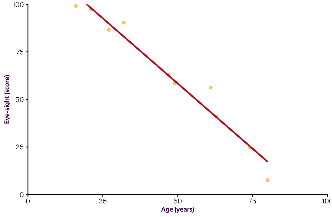
Figure 12.1: XX
Let’s first emphasise the connection between linear regression and ANOVA. For this we’ll use yet another linear regression example that we will then turn into a ANOVA–type problem. The question we’ll be investigating here is: Does Martian eye–sight depend on their age? For now, both variables (eye–sight and age) are continuous.
Figure 12.1 shows a scatter plot of the two variables, together with the regression line we get from OLS. As we know now this has the form \(f(X) = \hat \beta_0 + \hat \beta_1 X\), where \(\hat \beta_0\) and \(\hat \beta_1\) are the OLS estimates (determined by our data) of the underlying parameters \(\beta_0\) and \(\beta_1\) that describe the linear relationship between \(X\) and \(Y\) in the population. As in the previous chapter, our main interest here is to determine whether or not the observed value \(\hat \beta_1\) is big enough relative to the noise in the data so that we can reject the null hypothesis \(H_0: \beta_1 = 0\), i.e. the scenario where looking at age does not help when trying to predict the eye-sight of a Martian.
We probably all agree the scatterplot shows a lovely linear relationship between the two variables and that a lot can be said about the eye-sight of a Martian once we know their age. The linear regression output shown in Table 12.1 confirms this suspicion. The \(p\)–value for age is very small!
| Term | Estimate | Standard Error | Test statistic | p-value |
|---|---|---|---|---|
| \(\beta_0\) (intercept) | 126.9 | 5.2 | 25 | 0 |
| \(\beta_1\) (slope) | -1.4 | 0.1 | -14 | 0 |
Even before we formally carry out the \(t\)–test, we can guess that:
- the estimated value for \(\beta_1\) will be some negative number
- it will be large compared to it’s standard deviation
- the \(p\)–value for \(H_0: \beta_1 = 0\) will be small (this is a consequence of 1 and 2)
Table 12.1 also tells us that our best guess for the linear relationship between age and eye-sight has the form
\[ \text{(predicted eye-sight score when age} = x) = f(x) = 126.9 - 1.4 x,\]
i.e. for each year of age, the expected score for eye-sight decreases on average by 1.4 points.
As we learned in the previous chapter, the \(F\)–test provides another way to look at the problem. As opposed to the \(t\)–test, it doesn’t provide us with a formula for (our best guess of) the linear relationship between age and eye-sight, but it does look at the question of whether or not the variable age adds information when we try to explain the variation in eye-sight.
Table table below provides us with the output of the \(F\)–test for our example. As expected, we see a giant value for the \(F\)–statistic. This means that the residuals of the OLS solution are significantly smaller than the residuals for the horizontal null model. In other words, the improvement we get from taking age into account is a lot bigger than we’d expect if age didn’t play a role.
| Term | Degrees of freedom | Sum of the Squared… | Mean of the Squared… | Test statistic | p-value |
|---|---|---|---|---|---|
| Model | 1 | 8535 | 8535 | 188 | 0 |
| Residuals | 8 | 362 | 45 |
Now imagine that age was an ordinal instead of a continuous variable that consists of the categories youth, adult and senior.74 Figure 12.2 shows the new situation where \(X\) is a categorical variable with three levels. So far we have covered continuous \(X\) and categorical \(X\) with two levels in which cases you’d use linear regression and the two–sample \(t\)–test, respectively. Our new situation is sighly different and corresponds to a classical situation in which you’d use ANOVA!
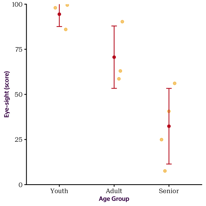
Figure 12.2: Transitioning from a continuous X variable to a categorical X variable with three levels.
Actually, ANOVA is an umbrella term for a family of methods. Here we will cover the simplest case which is called one–way ANOVA. One–way ANOVA answers the question if taking into account the levels of one categorical variable helps to explain the variation of a continuous variable.75 The statistical test that runs in the background when we perform ANOVA is the \(F\)–test that we already encountered. Moreover, we will show that the same analysis can also be carried out in a linear regression framework.
12.2 A simple example
Before we start looking at the actual Martian example, let’s first examine a simple dataset to observe the underlying concepts. The raw data are shown in the left–hand side of Figure . We have two variables, \(X\) and \(Y\), where \(X\) is a categorical variable with three groups, and \(Y\) is a continuous variable.
Remember, we can analyse the question whether or not the levels of \(X\) can help us explain the variation in \(Y\) either in the linear regression framework or with the \(F\)–test.
12.2.1 Linear regression with categorical explanatory variables
We first show how the data can be examined in a linear regression framework! In linear regression we were interested if we can find a line through the scatterplot of \(Y\) against \(X\) that better explains the data than the horizontal line that goes through the observed mean value \(\bar{y}\). Here, we are asking the same question except that it’s a bit meaningless to look for a straight line because \(X\) is not continuous and can only take three distinct values. So instead of looking for a line, we are asking whether or not we can find three group–specific \(y\)–values that are distinct from each other and (in terms of the residuals) fit the data better than just representing each group by the overall mean \(\bar{y}\).
As you can guess, the group–specific \(y\)–values that will fit the data better than the overall mean \(\bar{y}\) are the group mean values \(\bar{y}_1\), \(\bar{y}_2\) and \(\bar{y}_3\). However, the question is if this improvement is significantly better, i.e. if going the extra mile (reporting three instead of one value) is worth the effort.
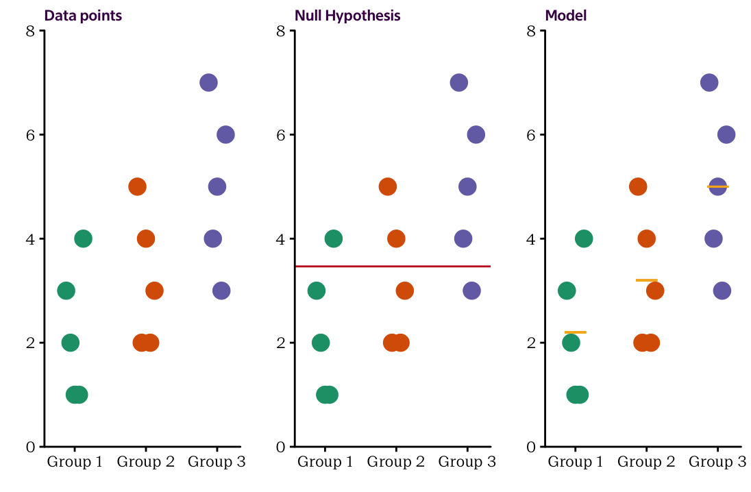
Figure 12.3: A fake dataset to help us explore the concepts in ANOVA. The data consist of a continuous variable described by three groups of a categorical variable.
Figure 12.3 displays the raw data and the two models we seek to compare. The middle plot shows the null model which is equal to the horizontal line through \(\bar{y}\), and the right hand side shows the plot with the three individual group means which takes the role of the OLS regression line in our situation. When we write down the two models as a formula, the null model is pretty simple:
\[\begin{eqnarray*} \hat{y}_i = \bar{y} & \text{ for all individuals $i$}. \end{eqnarray*}\]
The model we want to assess is a little bit more complicated as we need to distinguish between the three groups
\[\begin{eqnarray*} \hat{y}_i = \begin{cases} \bar{y}_1 & \text{if $i$th individual belongs to group 1} \\ \bar{y}_2 & \text{if $i$th individual belongs to group 2} \\ \bar{y}_3 & \text{if $i$th individual belongs to group 3} . \end{cases} \end{eqnarray*}\]
The distinction between the groups is a little annoying as the formula doesn’t look nice and concise. But luckily, with a bit of effort, we can rewrite it in a more compressed form as
\[ \hat{y}_i = \bar{y}_1 + (\bar{y}_2 - \bar{y}_1) \cdot x^{g2}_i + (\bar{y}_3 - \bar{y}_1) \cdot x^{g3}_i, \]
where the weird looking symbols \(x^{g2}_i\) and \(x^{g3}_i\) are so called indicator variables that take the values 0 and 1 to signify whether or not the \(i\)th individual belongs to group 2 and group 3, respectively.
For example if the 6\(th\) individual belongs to group 2, then \(x^{g2}_6 = 1\) and \(x^{g3}_6 = 0\) so that the whole equation becomes
\[\begin{eqnarray*} \hat{y}_6 & = & \bar{y}_1 + (\bar{y}_2 - \bar{y}_1) \cdot 1 + (\bar{y}_3 - \bar{y}_1) \cdot 0 \\ & = & \bar{y}_1 + (\bar{y}_2 - \bar{y}_1) \\ & = & \bar{y}_2. \end{eqnarray*}\]
Similarly, if the 11\(th\) individual belongs to group 3, then \(x^{g2}_{11} = 0\) and \(x^{g2}_{11} = 1\) so that the whole equation becomes
\[\begin{eqnarray*} \hat{y}_{11} & = & \bar{y}_1 + (\bar{y}_2 - \bar{y}_1) \cdot 0 + (\bar{y}_3 - \bar{y}_1) \cdot 1 \\ & = & \bar{y}_1 + (\bar{y}_3 - \bar{y}_1) \\ & = & \bar{y}_3. \end{eqnarray*}\]
If you understand the trick with the indicator variables, you actually understand the connection between ANOVA and linear models, because the only thing that’s left is a tiny substitution: if we replace \(\bar{y}_1\) by \(\hat{\beta}_0\), \((\bar{y}_2 - \bar{y}_1)\) by \(\hat{\beta}_1\) and \((\bar{y}_3 - \bar{y}_1)\) by \(\hat{\beta}_2\), our nice compressed equation above becomes \[\hat{y}_i = \hat{\beta}_0 + \hat{\beta}_1 x^{g2}_i + \hat{\beta}_2 x^{g3}_i,\]
which is just what we’d expect a linear model to look like! And we even know the values of the estimated coefficients already! In our little toy example \(\bar {y}_1 = 2.2\), \(\bar y_2 = 3.2\) and \(\bar y_3 = 5.0\), so that \(\hat{\beta}_0 = 2.2\) \(\hat{\beta}_1 = 1.0\) and \(\hat{\beta}_3 = 2.8\). With this, the entire regression equation becomes
\[\hat{y}_i = 2.2 + 1.0 \cdot x^{g2}_i + 2.8 \cdot x^{g3}_i. \]
Therefore the only thing left to close the circle with the linear regression as you know, is the \(t\)–test.
In the linear regression we were interested in the null hypothesis \(H_0: \beta_1 = 0\) because if we can reject this based on the data, it means that the OLS solution with the non-zero slope fits the data better than the null (horizontal) line. Here, we want to do the same thing, except that we are interested in two null hypotheses, namely \(H_0: \beta_1 = 0\) AND \(H_0: \beta_2 = 0\). If either one of them can be rejected based on the data, then we know that the group means are significantly different from each other. Hence, there is a significant improvement in taking group membership into account!
Table ANOVALM1 shows the computer output that we get when we apply linear regression to our data. The first value is the intercept which corresponds to \(\hat \beta_0\). The fact that it has a small \(p\)–value tells us that the mean of the first group is significantly different from zero. This is not the important point in our investigation because we are interested in the differences between the group means which are given by \(\hat \beta_1\) and \(\hat \beta_2\). The \(p\)–value for \(\hat \beta_2\) is quite large, so there is no evidence in the data that group 1 and group 2 have different mean values. However, the \(p\)–value for \(\hat \beta_2\) is very small. As \(\hat \beta_2\) measures the mean difference between group 1 and group 3, we have evidence that the observed difference is bigger than what we’d expect by pure chance! Therefore, we can conclude that the more complex linear model provides a better fit to the data than the null model.
12.3 Classical ANOVA
We said in the beginning of this chapter, we can carry out the same investigation with an \(F\)–test. Doing so would be the classical approach to assess mean differences for more than two groups. So when people talk about (one–way) ANOVA, this is what they probably mean. Let’s have a look at what the \(F\)–test does in our simple situation. Just like in the case where we compared two continuous variables against each other, the \(F\)–test works with the residuals of the two models under comparison.
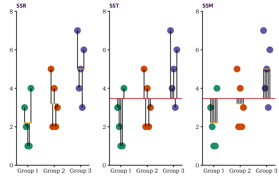
Figure 12.4: Three plots of our fake ANOVA dataset depicting SSR, SST and SSM, respectively. SSR considers the distance between each data point and the within–group mean, SST considers the distance between each data point and the grand mean of all data points, and SSM considers the distance between the within–group means and the grand mean.
| x | y | group-wise mean | global mean | y - group sq | y - grand sq | bar - group sq |
|---|---|---|---|---|---|---|
| 1 | 3 | 2.2 | 3.5 | 0.64 | 0.22 | 1.60 |
| 1 | 2 | 2.2 | 3.5 | 0.04 | 2.15 | 1.60 |
| 1 | 1 | 2.2 | 3.5 | 1.44 | 6.08 | 1.60 |
| 1 | 1 | 2.2 | 3.5 | 1.44 | 6.08 | 1.60 |
| 1 | 4 | 2.2 | 3.5 | 3.24 | 0.28 | 1.60 |
| 2 | 5 | 3.2 | 3.5 | 3.24 | 2.35 | 0.07 |
| 2 | 2 | 3.2 | 3.5 | 1.44 | 2.15 | 0.07 |
| 2 | 4 | 3.2 | 3.5 | 0.64 | 0.28 | 0.07 |
| 2 | 2 | 3.2 | 3.5 | 1.44 | 2.15 | 0.07 |
| 2 | 3 | 3.2 | 3.5 | 0.04 | 0.22 | 0.07 |
| 3 | 7 | 5.0 | 3.5 | 4.00 | 12.48 | 2.35 |
| 3 | 4 | 5.0 | 3.5 | 1.00 | 0.28 | 2.35 |
| 3 | 5 | 5.0 | 3.5 | 0.00 | 2.35 | 2.35 |
| 3 | 3 | 5.0 | 3.5 | 4.00 | 0.22 | 2.35 |
| 3 | 6 | 5.0 | 3.5 | 1.00 | 6.42 | 2.35 |
FakeDataTable The values used in our example ANOVA calculations.
Figure 12.4 shows the residuals of both the fitted model (left–hand–side) and the null model (middle). And similar to Figure XX in the previous chapter, it also displays the differences between the fitted and the null model (right). If you square each of the values and sum them up in each of the three cases, you get our dear friends \(SSR\), \(SST\) and \(SSM\), respectively. In our example, these quantities are:
| Term | Value |
|---|---|
| \(SSR\) | 23.6 |
| \(SST\) | 43.7 |
| \(SSM\) | 20.1 |
For reference, Table ?? shows all the values we are working with. Note that \(SSR\), \(SST\) and \(SSM\) are the sums of the values in columns 5–7.76
Have you noticed anything with the three sums of squares? Like before, we have the relationship
\[ SST = SSM + SSR, \]
so the total variation in the data, \(SST\), can be split into the variation that can be explained by fitting our model, \(SSM\), and the variation that we cannot do anything about, \(SSR\). As before, we could calcuate \(R^2 = SSM/SST\) as the proportion of the total variance that can be explained by our model. However, this number just gives us an impression whether or not or model fits the data significantly better than the null model. If we want a statistical test, we need to employ the \(F\)–test which compares \(SSM\) with \(SSR\). The corresponding output is shown in Table ??. This actually is the type of output you’ll usually encounter when ANOVA is performed.
In the table we see our familiar values \(SSM\) and \(SSR\), with the associated degrees of freedom \(df_1\) and \(df_2\). Like in the previous chapter, these numbers can be used to calculate the mean sum of squared for the model and the total, i.e.
\[MSM = \frac{SSM}{df_1} = \frac{ 20.1}{2} \quad \quad \text{and} \quad \quad MSR = \frac{SSR}{df_2} = \frac{23.6}{12}. \]
The ratio of these two numbers then gives the \(F\)–statistic. If it is large, we know that the variance explained by the model is large relative to the variance that remains after fitting it. In other words the group mean values are far apart from each other while the scatter of the original data points around the group mean values is small. Statisticians say “the variance between the groups is significantly larger than the variance within the groups.”77
You know the rest of the story already. To obtain the \(p\)–value, the observed value of the \(F\)–statistic is compared to the corresponding null distribution which is the \(F\)–distribution with \(df_1\) and \(df_2\) degrees of freedom. If it is large, there is not much area under the curve to the right of the observed \(F\)–statistic and the \(p\)–value is small. If it’s smaller than you chosen signficance level \(\alpha\), you can reject the null model with (\(1-\alpha\))% confidence.
Here the \(p\)–value is quite small, so it seems safe the reject the null model. But if linear regression and ANOVA are supposed to be the same, why do we only have one \(p\)–value on the ANOVA–type output while we had three in the linear regression output?! The answer is that linear regression looks at the data more closely and tests the diffrences between the individual groups (specifically, it tests the differences between group 1 and the other groups in turn) whereas the \(F\)–test takes a more unifying approach and examines the question whether there is at least one significant difference. So as a rule of thumb, if at least one \(t\)–test in the linear regression framework is significant (APART FROM THE ONE FOR THE INTERCEPT), then the \(F\)–test will also be.78
12.4 ANOVA on our Martian dataset
Let’s return to our burning question whether Martian age group has an influence on eye–sight. Here, we’ll do it the other way round and first use the \(F\)–test to take a global look at whether there are any differences in eye–sight between the age groups. If we do find any differences, then it is worth looking at the problem in a more detailed way to see where exactly the differences are.
| Term | Degrees of freedom | Sum of the Squared… | Mean of the Squared… | Test statistic | p-value |
|---|---|---|---|---|---|
| Model | 2 | 12851 | 6425 | 35 | 0 |
| Residuals | 17 | 3126 | 184 |
Table ?? shows the ANOVA output that contains the relevant information for the \(F\)–test. As expected from Figure 12.2, the model that fits different mean values for each age group offers a big improvement over the null model that fits all data points using the overall mean. The \(MSM\) is much bigger than the \(MSR\) so that we know that the variation of the eye–sight scores between the age groups is much bigger than the variation within the age groups. The observed \(F\)–statistic therefore takes an epic value of over \(34.94\) which obviously results in a very small \(p\)–value. So there basically is no chance that the null model is true and we observe group differences that are as big (or bigger) than the ones in our data.
The \(F\)–test confirms our visual suspicion that the differences between the groups are significant. Let’s put our linear regression glasses on and see where the differences are. Table ?? shows the corresponding output. It contains three very small \(p\)–values. The first \(p\)–value tells us the (not so interesting) fact that the underlying population mean of the eye–sight scores of the young Martians is significantly different from zero. The other two \(p\)–values are more interesting, since they tell us that both the adult and the senior Martians reveal eye–scores that are significantly different from the scores of the young Martians.
| Term | Estimate | Standard Error | Test statistic | p-value |
|---|---|---|---|---|
| \(\hat\beta_0\) (\(\bar{y}_{youth}\)) | 90 | 6.1 | 14.9 | 0.00 |
| \(\hat\beta_1\) (\(\bar{y}_{adult}\) - \(\bar{y}_{youth}\)) | -21 | 7.9 | -2.7 | 0.02 |
| \(\hat\beta_2\) (\(\bar{y}_{senior}\) - \(\bar{y}_{youth}\)) | -61 | 7.7 | -7.9 | 0.00 |
To find out if there are significant differences between the adult and the senior Martians you can carry out a separate \(t\)–test. Or you fit a different linear model where either the adult or the senior group is the reference group, which then corresponds to the intercept. A word of caution though: if you do many tests on the same dataset, you run into problems of multiple testing. That is beyond the scope of this course!
| Comparison | Difference in means | Lower 95 | Upper 95 | Adjusted p-value | |
|---|---|---|---|---|---|
| Adult-Youth | Adult-Youth | -21 | -42 | -0.79 | 0.04 |
| Senior-Youth | Senior-Youth | -61 | -81 | -41.55 | 0.00 |
| Senior-Adult | Senior-Adult | -40 | -58 | -22.22 | 0.00 |