5 Data Viz with ggplot2, themes
5.1 Built-in Themes
ggplot2 allows you to have fine control over all visual aspects of the plot. The default ggplot2 theme is theme_gray() (or theme_grey() will also work), but you can also choose theme_bw(), which produces a more minimalist plot. You can set the base size of a plot as an argument.
z <- ggplot(mtcars, aes(x = wt, y = mpg, colour = factor(cyl))) +
  geom_point(alpha = 0.6, size = 3, shape = 16) +
  scale_y_continuous("Miles/(US) gallon",
                     limits = c(10, 40),
                     breaks = seq(10, 40, 10),
                     expand = c(0,0)) +
  scale_x_continuous("Weight (lb/1000)",
                     limits = c(1,6),
                     breaks = 1:6,
                     expand = c(0,0)) +
  scale_colour_brewer("Cylinders")

z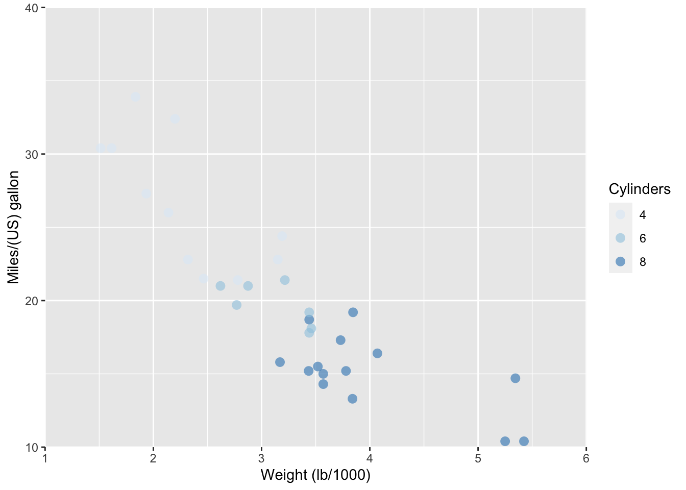
Figure 5.1: The ggplot2 default theme_gray() and magnified theme_bw().
# Black and White theme, with larger base size, shown right:
z + theme_classic(12)
5.2 Custom themes:
You can change individual aspects by modifying the default template, as shown below.
# Custom theme, shown right:
z + theme(rect = element_blank(),
          axis.ticks = element_line(colour = "#A50F15"),
          axis.text = element_text(colour = "#A50F15"))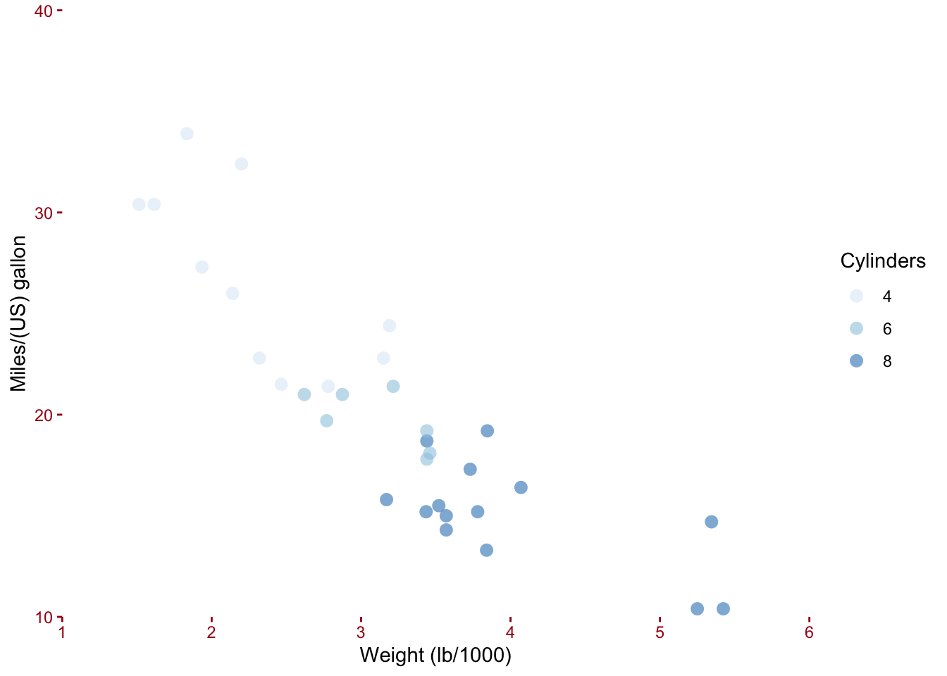
Figure 5.2: An example of updating an individual ggplot with custom theme settings using the theme() function.
Arguments for the themes layer in ggplot2 v 3.2.1:
Text, modify with element_text()
-
text-
titlelegend.titleplot.titleplot.subtitleplot.captionplot.tag
-
axis.title-
axis.title.xaxis.title.x.topaxis.title.x.bottom
-
axis.title.yaxis.title.y.leftaxis.title.y.right
-
-
axis.text-
axis.text.xaxis.text.x.topaxis.text.x.bottom
-
axis.text.yaxis.text.y.leftaxis.text.y.right
-
legend.text-
strip.textstrip.text.xstrip.text.y
-
Lines, modify with element_line()
-
line-
axis.ticks-
axis.ticks.xaxis.ticks.x.topaxis.ticks.x.bottom
-
axis.ticks.yaxis.ticks.y.leftaxis.ticks.y.right
-
-
axis.line-
axis.line.xaxis.line.x.topaxis.line.x.bottom
-
axis.line.yaxis.line.y.leftaxis.line.y.right
-
-
panel.grid-
panel.grid.majorpanel.grid.major.xpanel.grid.major.y
-
panel.grid.minorpanel.grid.minor.xpanel.grid.minor.y
-
-
Rect, modify with element_rect()
-
rectlegend.backgroundlegend.keypanel.backgroundpanel.borderplot.background-
strip.backgroundstrip.background.xstrip.background.y
Units, specify with unit()
-
axis.ticks.length-
axis.ticks.length.xaxis.ticks.length.x.topaxis.ticks.length.x.bottom
-
axis.ticks.length.yaxis.ticks.length.y.leftaxis.ticks.length.y.right
-
-
legend.spacinglegend.spacing.xlegend.spacing.y
-
legend.key.sizelegend.key.heightlegend.key.width
legend.box.spacing-
panel.spacingpanel.spacing.xpanel.spacing.y
plot.marginstrip.switch.pad.gridstrip.switch.pad.wrap
Positioning and sizes
aspect.ratiolegend.marginlegend.text.alignlegend.title.alignlegend.positionlegend.directionlegend.justification-
legend.boxlegend.box.justlegend.box.marginlegend.box.background
panel.ontopplot.tag.positionstrip.placement
When creating new themes from scratch:
-
complete,TRUEif this is a complete theme, e.g.theme_grey(). Complete themes behave differently when added to a ggplot object. All elements will be set to inherit from blank elements. Defaults toFALSE. -
validate,TRUEto run validate_element(), defaults toFALSE.
It’s common to combine your custom theme with a built in theme:
# Custom theme, shown right:
z + theme_classic() +
  theme(rect = element_blank(),
          axis.ticks = element_line(colour = "#A50F15"),
          axis.text = element_text(colour = "#A50F15"))
Which can also be saved as its own layer:
myTheme <- theme_classic() +
  theme(rect = element_blank(),
          axis.ticks = element_line(colour = "#A50F15"),
          axis.text = element_text(colour = "#A50F15"))

z + myTheme
5.3 Updating the default theme:
# Save theme_gray() settings, and make an update:
original <- theme_update(panel.background = element_blank(),
                         legend.key = element_blank(),
                         axis.line = element_line(colour = "black"),
                         legend.position = c(.9, .9),
                         panel.grid.major = element_blank(),
                         panel.grid.minor = element_blank(),
                         axis.title.x = element_text(vjust = -0.3),
                         axis.text.x = element_text(colour = "black"),
                         axis.text.y = element_text(colour = "black")
                         )
# Plot with updated theme_gray() theme, shown left
z
# Reset original theme_gray() settings
theme_set(original)
# Plot with original theme_gray() settings, shown right
z