Chapter 17 Element 8: Regular Expressions
17.1 Learning Objectives:
By the end of this chapter you should know what
- Regular expressions are,
- How to compose them, and
- How to use
grep()and thestringrpackage
Regular expressions are codes that identify certain patterns in a string of text. A biological analogy would be using BLAST to search for a short DNA sequence in the genome. The difference is that instead of letting an algorithm (e.g. BLAST) decide the best match, we specify the precise matching rules in the search pattern. This means that regular expressions are strictly defined, making them very powerful when used correctly, or potentially useless if not.
For example, refering back to our protein_df examples, surprisingly simple regular expressions will allow us to clean up our Uniprot labels so that we can produce such plots:
source("data/genes.R")As an example, we will consider some gene sequences provided for the workshop. Source the “genes.R” file:
source("data/genes.R")You should now have a vector called genes with 50 elements.
length(genes)# [1] 50We can find out if a gene contains a specific restriction site (e.g. GGGCCC).
which(genes=="GGGCCC")# integer(0)In this case we need to search for a character string as a part of another character string. grep() performs pattern matching.52
grep("GGGCCC",genes)# [1] 5The 5\(^{th}\)53 element contains the string GGGCCC. However, grep() can also more elaborate regex codes to match the same pattern. These codes are regular
expressions. For example, we can use G\{3\}C\{3\}54instead
of GGGCCC:
grep("G{3}C{3}",genes)# [1] 5The power of this technique becomes apparent when we introduce some ambiguity into our sequence. For example, if we just wanted G followed by any 4 characters and a C, we can use:
grep("G.{4}C",genes)# [1] 1 2 3 4 5 6 7 8 9 10 11 12 13 14 15 16 17 18 19 20 21
# [22] 22 23 24 25 26 27 28 29 30 31 32 33 34 35 36 37 38 39 40 41 42
# [43] 43 44 45 46 47 48 49 50The dot (.) means to look for any character.
The 5\(^{th}\) element is found again, but this time many more elements match our search criteria because it is ambiguous.
You can imagine how convenient regular expressions are when you want to find precise information in a large data-set. Regular expressions allow you to discover not only if a given pattern is present, but also where it is, and what the matching text is. You can also replace matching text using sub().
In addition to grep() and sub() in the base package, the functions provided by the stringr package are very useful. The most common functions for working with regular expressions are listed in table 17.1.
| Function | Description |
|---|---|
grep(), grepl() |
Which strings contain the pattern? Detect presence of a pattern, returning the index number which can be used as an index. |
sub() |
Can I substitute the matched string? Replace the first matched pattern, returning a character vector. |
stringr::str_detect() |
Which strings contain the pattern? Detect presence/absence of a pattern, returning a logical vector which can be used as an index. |
stringr::str_locate() |
Where in the string is the pattern? Locates the first position of a pattern, returning a numeric matrix with the start and end value. |
stringr::str_extract() |
What is the string that matches the pattern? Extract the text corresponding to a pattern, returning a character vector. |
stringr::str_match() |
What are the sub-sets of the matched pattern? Extracts sub-groups defined by () in the pattern, returning a character matrix of the group and all sub-groups. |
stringr::str_replace() |
Can I substitute the matched string? Replace the first matched pattern, returning a character vector. |
stringr::str_split_fixed() |
Can I separate the string into separate items? Split the string into a fixed number of pieces based on the pattern, returning a character matrix |
Now that you are familiar with the concept of regular expressions as a set of codes, we’ll work with a small data-set, to show how to use them to analyse your own data. Table 17.2 provides a list of the most common codes.
| Type | Symbol | Matching Pattern |
|---|---|---|
| Anchors | ^ |
Start of string |
$ |
End of string | |
| Character Classes | \\s |
White space |
\\S |
Not white space | |
\\d |
Digit | |
\\D |
Not digit | |
\\w |
Word | |
\\W |
Not word | |
| Quantifiers | * |
0 or more |
*? |
0 or more, ungreedy | |
+ |
1 or more | |
+? |
1 or more, ungreedy | |
? |
0 or 1 | |
?? |
0 or 1, ungreedy | |
{4} |
Exactly 4 | |
{4,} |
4 or more | |
{4,6} |
4, 5 or 6 | |
{4,6}? |
4, 5 or 6, ungreedy | |
| Ranges | . |
any character |
(a|b) |
a or b | |
[abc] |
a, b or c | |
[^abc] |
Not a, b or c | |
[p-z] |
Lower-case letter between p and z | |
[P-Z] |
Upper-case letter between P and Z | |
[3-6] |
Digit between 3 and 6 | |
[a-zA-Z] |
Alphabetic characters | |
[^a-zA-Z] |
Non-alphabetic characters | |
[a-zA-Z0-9] |
Alphanumeric characters |
We’ll begin by making a small character vector to use as our search space:
Note that grep() and str_detect() have different syntax (i.e. argument order) and provide different vectors as output. grep() returns the matching element’s position in the vector, whereas str_detect() returns a full logical vector. grep() already provides the exact location of the matches. If we wanted to use stringr functions, the command would be: which(str_detect(genes, "53")). Although stringr functions are more simple in some respects, this is not the case here. grep() is still a valuable function to learn. Here, we use the logical vector returned from str_detect() as an index to obtain the actual values. We could have also used the output from grep() in the same way.
Here, we use the logical vector returned from str_detect() as an index to obtain the actual values. We could have also used the output from grep() in the same way.
genes <- c("alpha4", "p53", "CDC53", "Agft-4", "cepb2")
genes
# [1] "alpha4" "p53" "CDC53" "Agft-4" "cepb2"# Use grep to find the position of all values in the "genes" vector that contain "53" at any position.
grep("53", genes)# [1] 2 3# Initialize the {stringr} package
library(stringr)
# Use str_detect to find the position of all values in the "genes" vector that contain "53" at any position.
str_detect(genes, "53")# [1] FALSE TRUE TRUE FALSE FALSEThe syntax for extracting the exact values of the matching elements can be tricky with grep(). The stringr package simplifies this process.
genes[str_detect(genes, "53")]# [1] "p53" "CDC53"# Search for all elements in "genes" that begin with "C".
str_detect(genes, "^C")# [1] FALSE FALSE TRUE FALSE FALSE# Search for all elements in "genes" that begin with "C" or "c".
str_detect(genes, "^(C|c)")# [1] FALSE FALSE TRUE FALSE TRUESimilar to the logical operators we have already used in R, regular expressions use | to denote or.
# Alternatively:
str_detect(genes, regex("^C", ignore_case = TRUE))
# [1] FALSE FALSE TRUE FALSE TRUE# Search for all elements in "genes" that begin with a "C" or "c" and end with a number:
str_extract(genes, regex("^c.*\\d$", ignore_case = TRUE))# [1] NA NA "CDC53" NA "cepb2"# But contrast this with:
str_extract(genes, "53")# [1] NA "53" "53" NA NANote how str_extract() does not return the whole matching element, but rather just that part which matches the regular expression.
# extract only those elements in "genes" that begin with a "C" or "c" and end with a number:
genes[str_detect(genes, regex("^c.*\\d$", ignore_case = TRUE))]
# [1] "CDC53" "cepb2"# Search for all elements in the "genes" vector that end with "53".
str_detect(genes, "53$")# [1] FALSE TRUE TRUE FALSE FALSE# Search for all elements in the "genes" vector that begin with a letter.
str_detect(genes, "^[a-zA-Z]")# [1] TRUE TRUE TRUE TRUE TRUE#Alternatively:
str_detect(genes, "^\\w")# [1] TRUE TRUE TRUE TRUE TRUE# Replace all occurrences of "53" in "genes" with "XX"
str_replace(genes,"53","XX")# [1] "alpha4" "pXX" "CDCXX" "Agft-4" "cepb2"17.2 Working with Strings
R features several functions for working with strings that are useful when reporting results. See table 17.3.
| Function | Description |
|---|---|
paste(..., sep="") |
Create a sentence, specify separator with sep argument. |
paste0(...) |
Create a sentence, defaults to no separator between pieces. |
toupper(x) |
Convert to upper-case. |
tolower(x) |
Convert to lower-case. |
The power of regular expressions will become clear when applied to the protein_df data frame. For this we will consider the Description column to search for some key words.
Exercise 17.1
To make writing code easier, we will save the search area in a new object. In this case the search area is the Description variable (i.e. column). Save it in a new object called desc.
- Print out the
Descriptionwhich contain the string “methyl.” - What are the actual positions (i.e. rows) that contain “methyl?”
- How many matches are there to the string “methyl?”
- Write a logical expression that tells us if case insensitivity makes a difference in searching for the string “methyl.”
Exercise 17.2 Since str_detect() results can be used as an index, we’ll use it to look at the HM ratios of all our genes of interest.
- First, search the
protein_df$Descriptionfor all mentions of “ubiquitin” and save this index asubi: - Then use this index to access values in the transformed
Ratio.H.Mvariable. - Create a new data frame containing only the names, H/M, and M/L ratios for ubiquitin proteins.
Exercise 17.3 Using the material discussed so far in the workshop, can you generate the following plot which compares the “ubiquitin” protein ratios in HM and ML conditions?
The commands used are provided below. We begin with the protein_df data frame containing the transformed and normalised Ratios and directly lead into our plotting functions. There are 5 values you need to fill in.
protein_df %>%
  filter(str_detect(___1___, regex("___2___", ignore_case = T))) %>%
  select(___3___, ___4___, ___5___) %>%
  filter(complete.cases(.)) %>%
  ggplot(aes(___4___, ___5___)) +
  geom_point() +
  labs(title = "Only Ubiquitins")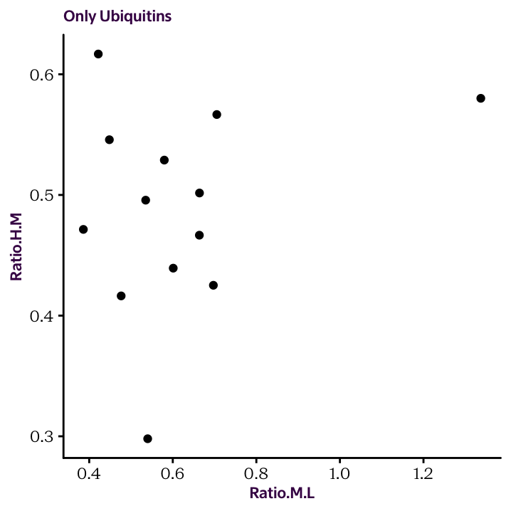
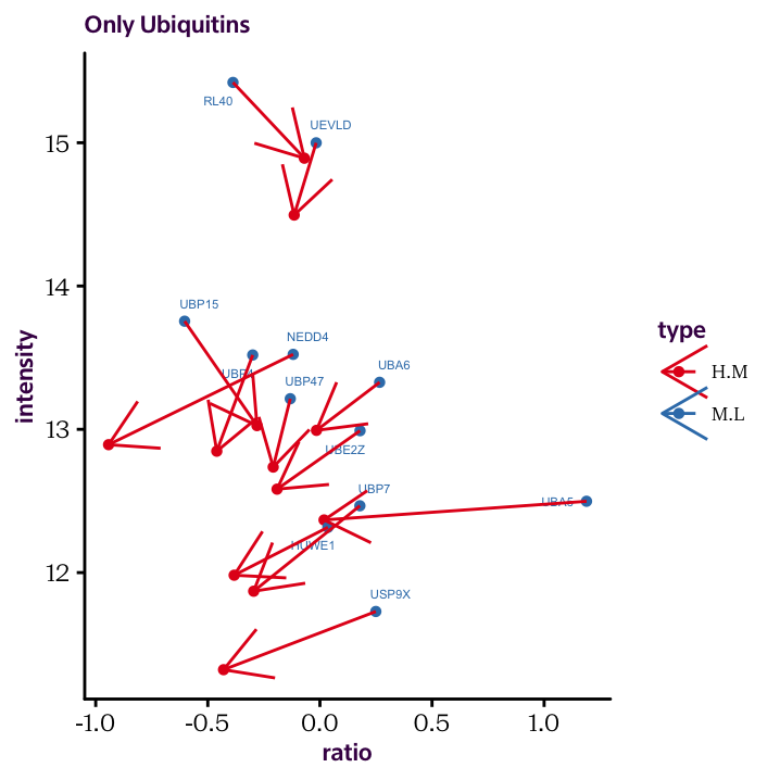
As an extension of the previous example, see if you can generate the following plot, which puts both ratios on the x axis and shows the connection between the two conditions with an arrow.
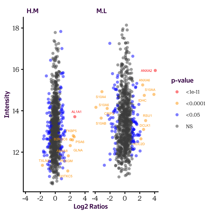
The code to produce the plot presented at the beginning of this chapter is presented below. We produced the allData data frame in the previous chapter. Here, I’m using the ggrepel package to displace the Uniprot labels a small amount so that they don’t overlap the dots.
library(ggrepel)                                                                         # Load package
ggplot(allData, aes(Expression, Intensity, col = SigCat)) +                              # Establisth plot base layer
  geom_point(alpha = 0.5, shape = 16) +                                                  # Geom point layer
  geom_text_repel(data = allData[allData$SigCat %in% c("<1e-11", "<0.0001"),],           # Geom test layer specifying subset of data
                  aes(label = sub("_.*$", "", Uniprot)), size = 1.5, show.legend=F) +    # Aesthetics for text
  scale_colour_manual(limits = c("<1e-11", "<0.0001", "<0.05", "NS"),                    # Set labels on color scale
                      values = c("red", "orange", "blue", "grey30")) +
  labs(x = "Log2 Ratios", y = "Intensity", col = "p-value") +                            # Set axis labels
  facet_grid(. ~ Ratio)                                                                  # Split plot according to Ratio
The name grep has been carried over from the original application on the Unix operating system. It stands for global/regular expression/print, which means: search a data-set globally (i.e. everywhere) for a regular expression and print the lines containing a match.↩︎
Note that the element number, and not the element itself is returned.↩︎
{3}means to look for exactly 3 of the preceding term.↩︎