Chapter 8 Case-study: SILAC

Now that we’re familiar with some of the basic concepts of functional and object-oriented programming, let’s work on some real data!

8.1 Importing Data

It is likely that most of your data is found in an Excel or tab-delimited table, like the text files provided for the workshop. Use these base package functions to import your data and save them as a variable.

Table 7.3: Base package functions for importing data. These functions will handle most of your general input/output needs.
Function	Description
`read.table(file)`	Read file in table format into data frame.
`read.csv(file)`	Read comma-separated data.
`read.csv2(file)`	Read semicolon-separated data.
`read.delim(file)`	Read tab-delimited data into data frame.
`read.delim2(file)`	Read tab-delimited data where the decimal place is a `,`.

8.1.0.1 stringsAsFactors

An important thing to consider here is something that I mentioned at the end of the dataframes section, 7.3.2.1. R version 4.0, released (April, 2020), changed the default value of these import functions. The argument stringsAsFactors is now FALSE by default, istead of TRUE. If you use these functions in older versions of R, columns that contain characters will be converted to factors. We’ll discuss factors in 11.

This behavior was for a good, but out-dated, reason and became a long-standing complaint in the R community. Although the community wanted to have this default behavior changed, it does create some confusion since you may inherit old R scripts from colleagues that are aware of this behavior and utilize factors in their script. If you run those scripts using an upgraded version of R, you may encounter problems.

An alternative to the base package functions given above, the readr package, part of the tidyverse, can make things easier and faster in some cases. In particular, it doesn’t convert characters to factors when importing, so older and newer scripts will work in the same way.

Table 8.1: `readr` package functions for importing data.
Function	Description
`read_csv()`	Read comma-separated data.
`read_csv2()`	Read semicolon-separated data.
`read_tsv()`	Read tab-delimited data.
`read_delim()`	Reads data with any delimiter.

The rio package (R Input/Output) offers the import() function for generic import of many different file formats. This is a good starting point if you are going to read in an Excel file. Nonetheless, I would encourage you to not begin working in R using Excel files. It’s my experience that the Excel files that students like to use are often times contaminated with summary statistics, multiple tables, plots, colors & lines that encode information, multiple worksheets and inconsistent use of white space. All of these things can be dealt with in R, but they make your life more difficult than it needs to be. Learning R is already a lot of work, so make your life easier by starting with a dataset that that is going to be easy to read into R and has not been modified after it was generated.

The Protein.txt file, contains protein expression data in the form of ratios and signal intensities. There are 15 variables (i.e. columns) in the data frame. Proteins were labelled with stable isotopes of heavy or medium mass difference to the normal (low) protein mass. This leads to three ratios for each protein:

H/M - High:Medium weight
M/L - Medium:Low weight
H/L - High:Low weight

In addition, the intensity of each peptide, for each label, was recorded when the proteins were analysed by mass spectrometry. Individual peptide intensities have already been combined to give 3 label intensities for each protein.

Exercise 8.1 (Import and Examine) Here we are going to use the RStudio cloud platform. So I know that the file to import is in your working directory.

If you set up a new project in RStudio Desktop, then you can move your data files into that folder on your computer and they will also be in your working directly.

Import the tab-delimited file called Protein.txt, found inside the data folder, and save it as an object called protein_df. See the notes below if your having a hard time.

A very common point of confusion is what should be the argument for any of the import functions given above. Many students just do something like:

read.delim(Protein.txt)

This will produce an error saying that the protein.txt object is not found. That makes perfect sense because you gave an argument pointing to some object in your environment not to a file on your computer (or in this case the cloud). So you need to give the name of the file using "", and more than that, you need to specify which sub-directory it’s in. Try "data/Protein.txt"

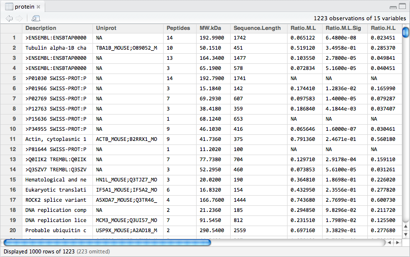
Exercise 8.2 (Examine structure) What type of data is contained in each column? Use some of the functions we introduced in the dataframes section.

Figure 8.1: The protein_df data frame.

Typically, the first step is to clean up the data-set. In this case that would mean removing contaminants. However, we’re going to focus on applying tools we’re already familiar with and get to that in the next section. But, there are many ways to go about applying transformations to your data set. Here we can use older base package methods. The reason I show this is because it’s very simple and you will see it a lot in help pages and scripts, so it’s worthwhile being familiar with both base package and tidyverse ways of doing things.

Exercise 8.3 (Clean-up and Transform I) There are three intensity columns, corresponding to the H, M and L labelled proteins: - Intensity.H - Intensity.M - Intensity.L

Intensities are typically transformed to a \(log_{10}\) scale. Perform a \(log_{10}\) transformation on each intensity column and replace the existing columns in situ with their transformed values.

Exercise 8.4 (Clean-up and Transform II) Since we’re working with ratios, a protein’s intensity is actually the sum of each label’s intensity. Calculate the sum of each combination of \(log_{10}\) intensities, H+M and M+L (we’re not interested in H+L), and store them in new columns called Intensity.H.M and Intensity.M.L, respectively.

Exercise 8.5 (Clean-up and Transform III) Perform a \(log_2\) transformation of the ratios and store the values in situ in the same columns.

Next, confirm that protein_df has the correct dimensions, column names and information:

# New dimensions of the data frame:
dim(protein_df)

# [1] 1223   17

# The first 6 values of log2.rat.HM
head(protein_df$Ratio.H.M)

# [1] -1.5105 -1.0003 -1.1532 -1.0851      NA -0.0046

8.2 Saving a data frame to a file

There are several ways to save an R object outside of the environment. If you have a data frame, The most straightforward way is to use the rio package:

Function	Description
`export(df, file)`	Save the data frame `df` as a file.

This will save the file type according to the file extension. For example, "myData.txt" will result in a tab-separated file.

Alternatively, you’ll also see base package versions:

Function	Description
`write.table(df, file)`	Save the data frame `df` as a file.
`write.csv(df, file)`	Save the data frame `df` as a comma-separated file.
`write.csv2(df, file)`	Save the data frame `df` as a semicolon-separated file.

Try using the form write.table(df, "data.txt", sep = "\t", row.names = F) to produce tab-delimited files. You can see that export() takes care of a lot of the settings for you, just by giving a proper extension to your file.