Chapter 10 Element 4: Indexing

10.1 Learning Objectives

By the end of this chapter you should be familiar with:

Indexing using [], and

We already encountered a type of indexing when we used the subset() function and logical expressions. Here, we will go one step further and perform indexing without using any unnecessary functions. We can filter our data-set according to:

Equations (i.e. using logical expressions, see section 9
Position (i.e. using row & column number, discussed here.), or
Text matching (i.e. using regular expressions).

10.2 Indexing vectors (1D)

The beauty of indexing is that we can use [] notation for all of these types of questions. We can limit our investigation to specific data points by using the [x] notation to select the $x{}^{th}$ data point in a vector. Let’s return to the simple foo1 example.

foo1         # Our data-set

#  [1]  1  8 15 22 29 36 43 50 57 64 71 78 85 92 99

foo1[6]    # The value at position 6

# [1] 36

p            # An object to use for indexing

# [1] 6

foo1[p]    # The value at position p

# [1] 36

foo1[3:p]  # The values between position 3 and p

# [1] 15 22 29 36

foo1[3:length(foo1)] # Position 3 to the end of foo1

#  [1] 15 22 29 36 43 50 57 64 71 78 85 92 99

This is convenient, but becomes very powerful when we start mining our data by combining position with logical expressions. Recall that the result of a logical expression is a TRUE/FALSE answer, which can be used as an index.

# For every value in foo1, is it less than 50?
foo1 < 50

#  [1]  TRUE  TRUE  TRUE  TRUE  TRUE  TRUE  TRUE FALSE FALSE FALSE
# [11] FALSE FALSE FALSE FALSE FALSE

# Save the logical expression as an object and use it
# as an index to report only the TRUE results
m <- foo1 < 50
foo1[m]

# [1]  1  8 15 22 29 36 43

# Use the logical expression as an index to report
# only the TRUE results
foo1[foo1<50]

# [1]  1  8 15 22 29 36 43

# Combine logical expressions to find values:
# Either less than or equal to 22 or greater than 71
foo1 <= 22 | foo1 > 71

#  [1]  TRUE  TRUE  TRUE  TRUE FALSE FALSE FALSE FALSE FALSE FALSE
# [11] FALSE  TRUE  TRUE  TRUE  TRUE

# How many are there:
sum(foo1 <= 22 | foo1 > 71)

# [1] 8

# What are they?
foo1[foo1 <= 22 | foo1 > 71]

# [1]  1  8 15 22 78 85 92 99

10.3 Indexing Dataframes (2D)

Recall that each column in a data frame is the same as a vector. Returning to the foo_df data frame we defined earlier, let’s try to extract the same information using logical expressions instead of the subset() function.

# Our data frame
foo_df

#   healthy    tissue quantity
# 1    TRUE     Liver        1
# 2   FALSE     Brain        7
# 3   FALSE    Testes       13
# 4    TRUE    Muscle       19
# 5    TRUE Intestine       25
# 6   FALSE     Heart       31

# The tissue variable (i.e. column, vector)
foo_df$tissue

# [1] "Liver"     "Brain"     "Testes"    "Muscle"    "Intestine"
# [6] "Heart"

# Which rows specify Liver?
# First make an index
foo_df$tissue == "Liver"

# [1]  TRUE FALSE FALSE FALSE FALSE FALSE

# Which values in the index are TRUE
which(foo_df$tissue == "Liver")

# [1] 1

# How many Liver samples are there?
# TRUE values = 1, so take the sum.
sum(foo_df$tissue == "Liver")

# [1] 1

Notice that we can combine an index of one column (i.e. foo_df\$healthy == TRUE) to extract values from another (foo_df\$quantity).

# The quantity values of only healthy observations
foo_df$quantity[foo_df$healthy == TRUE]

# [1]  1 19 25

To really make use of indexing with data frames, we can use [x,y] notation to select the $x{}^{th}$ row (i.e. observation) of the $y{}^{th}$ column (i.e. variable).

# The fourth row (i.e. observation)
foo_df[4,]

#   healthy tissue quantity
# 4    TRUE Muscle       19

# The fourth row, second column (i.e. variable)
foo_df[4,2]

# [1] "Muscle"

10.4 Exercises for Indexing

With the tools we have introduced so far, you will be able to start data mining. Let’s begin by extracting some interesting information from the protein_df data frame. First, let’s return to the exercises from the previous chapters and see if you can answer these questions in an easier way now:

Exercise 10.1 (Find protein values) Given a list of Uniprot IDs:

GOGA7
PSA6
S10AB

Find the corresponding $log_{2}$ ratios for each of the three conditions (H/M, M/L, H/L). Don’t use filter(), use [] instead.

Exercise 10.2 (Find significant hits) For the H/M ratio column, create a new data frame containing only proteins that have a p-value less than 0.05. Don’t use filter(), use [] instead.

Exercise 10.3 (Find extreme values) For the H/M ratio column, create a new data frame containing only proteins that have a $log_{2}$ ratio above 2.0 or below -2.0. Again, try to determine this without creating a new data set or using the subset() function.

The following sections will help you to answer the previous exercises

10.5 Ordering functions

There are a couple different ways to think about sorting data. Don’t confuse the following functions:

Table 10.1: Examples of some simple and frequently used functions for reordering data.
Function	Description
`sort()`	Returns a sorted vector (ascending or descending). Calls `order()` under-the-hood.
`order()`	Returns an index (integer vector) of the position of the ordered values (ascending or descending). Use this for data frames. Allows ordering on multiple vectors.
`rank()`	Returns the ranks of values in a vector, e.g. in non-parametric tests.
`arrange()`	Part of the `tidyverse`. Rearranges a variable

# A vector (or a variable in a data frame):
foo3

# [1] "Liver"     "Brain"     "Testes"    "Muscle"    "Intestine"
# [6] "Heart"

sort(foo3) # values after ordering

# [1] "Brain"     "Heart"     "Intestine" "Liver"     "Muscle"   
# [6] "Testes"

order(foo3) # index position after ordering

# [1] 2 6 5 1 4 3

foo3[order(foo3)] # i.e. sort()

# [1] "Brain"     "Heart"     "Intestine" "Liver"     "Muscle"   
# [6] "Testes"

foo_df

#   healthy    tissue quantity
# 1    TRUE     Liver        1
# 2   FALSE     Brain        7
# 3   FALSE    Testes       13
# 4    TRUE    Muscle       19
# 5    TRUE Intestine       25
# 6   FALSE     Heart       31

foo_df %>% 
  arrange(tissue)

#   healthy    tissue quantity
# 1   FALSE     Brain        7
# 2   FALSE     Heart       31
# 3    TRUE Intestine       25
# 4    TRUE     Liver        1
# 5    TRUE    Muscle       19
# 6   FALSE    Testes       13

foo_df %>% 
  arrange(desc(tissue))

#   healthy    tissue quantity
# 1   FALSE    Testes       13
# 2    TRUE    Muscle       19
# 3    TRUE     Liver        1
# 4    TRUE Intestine       25
# 5   FALSE     Heart       31
# 6   FALSE     Brain        7

10.5.1 Exercise for ordering

Exercise 10.4 (Find top 20 values) Which proteins (i.e. Uniprot IDs) have the 20 highest $log_{2}$ H/M and M/L ratios?

10.6 Intersection functions

To answer the last exercise you’ll need to know a bit about combining data. We saw merge functions in the section on data frames (page 7.4). Here, is another set of functions which is very useful: the intersect family. Given vectors x and y:

Table 10.2: The `intersect()` family of functions.
Function	Description
`intersect(x, y)`	Values in both vectors `x` and `y`.
`setdiff(x, y)`	Values in vector `x`, which are not in `y`.
`setdiff(y, x)`	Values in vector `x`, which are not in `y`.
`union(x, y)`	Set of all unique values in vectors `x` and `y`.

xx <- 1:8
yy <- 5:12

intersect(xx, yy)

# [1] 5 6 7 8

setdiff(xx, yy)

# [1] 1 2 3 4

setdiff(yy, xx)

# [1]  9 10 11 12

union(xx, yy)

#  [1]  1  2  3  4  5  6  7  8  9 10 11 12

10.6.1 Exercise for Intersections

Exercise 10.5 (Find intersections) Which proteins appear in the top twenty lists of both HM and ML?

10.7 Performing Statistical Tests

R is extremely powerful when it comes to performing statistical tests. Here, we will do a Pearson’s correlation between the Log2 ratios of HM and HL. The correlation test will be done with the cor.test() function, as follows:

⁴³

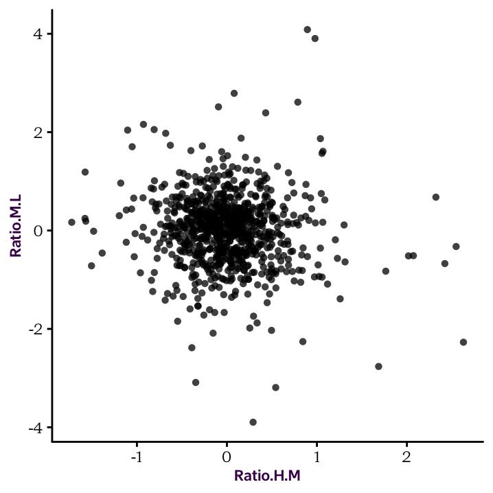
HM.ML.cor <- cor.test(protein_df$Ratio.H.M,
                      protein_df$Ratio.M.L)
HM.ML.cor

# 
#   Pearson's product-moment correlation
# 
# data:  protein_df$Ratio.H.M and protein_df$Ratio.M.L
# t = -3, df = 830, p-value = 0.01
# alternative hypothesis: true correlation is not equal to 0
# 95 percent confidence interval:
#  -0.156 -0.021
# sample estimates:
#    cor 
# -0.089

The cor.test() function provides a set of values which can be individually accessed:

# HM.HL.cor
attributes(HM.ML.cor)

# $names
# [1] "statistic"   "parameter"   "p.value"     "estimate"   
# [5] "null.value"  "alternative" "method"      "data.name"  
# [9] "conf.int"   
# 
# $class
# [1] "htest"

class(HM.ML.cor)

# [1] "htest"

names(HM.ML.cor)

# [1] "statistic"   "parameter"   "p.value"     "estimate"   
# [5] "null.value"  "alternative" "method"      "data.name"  
# [9] "conf.int"

HM.ML.cor$p.value

# [1] 0.01

HM.ML.cor$estimate # R

#    cor 
# -0.089

HM.ML.cor$estimate^2 # R-squared

#   cor 
# 0.008

The class of a cor.test() output is htest (hypothesis test). htest objects are lists. They have some unique properties, but you can extract information in a similar way as in data frames.

Note that the default cor.test() function performs a Pearson correlation coefficient. If we wanted to perform a Spearman’s rank-correlation coefficient, we would have to set the method argument to "spearman". Also, in the output, cor refers to $R$. To calculate the more common $R^2$, you will have to square it.↩︎