Chapter 3 A Journey to Mars … and some problems …
Throughout this workshop we’ll use a hypothetical scenario to introduce the key concepts in statistics: a journey to Mars (yes, Mars!7 ). The story begins as such:
Our story takes place in the near future. Scientists have been pretty excited about going to Mars since they spotted some Martians wandering about on the surface! Obviously, they want to know everything about them, so a mission was sent to collect 20 Martians and bring them back to Earth. Back on Earth, you are the lucky scientist tasked with making the first observations - and so we begin…
3.1 Samples and Populations
The group of 20 Martians that we take home to Earth is a sample, and they are collected from the entire population of Martians.
A population is loosely defined as any collection of individuals in which we may be interested.
A sample is a group of individuals taken from a population – usually for the purpose of a scientific investigation of the underlying population.
Some examples of populations:
- All Martians on Mars
- All German females with type II diabetes over the age of 45
- All wild boars in Grunewald forest in Berlin
- All B cells in a mouse
- The blood pressure of all men at any given time
Note from these examples that the individuals we’re interested in can be anything. Usually the size of the sample is much smaller than that of the population because we almost always have the situation where it’s impossible to study the entire population. In many cases this is because it would take too much time or it would be to costly. Sometimes our population is even infinitly large, so that even with all the time and the money in the world, we couldn’t possibly study all the individuals in the population.
Exercise Which of the populations above can be described as infinite?
Exercise Give an example of a population of interest in your own research.
Exercise Imagine that you are an experimental biologist. You have just generated a new mouse line with a specific genotype and therefore, you have all mice in existence with this genotype in your hands. What’s the population of interest in this case?
These exercises show that, although the definitions of sample and population may seem obvious at first glance, there are a few subtleties involved. To make things worse, there is one more distinction that we want to draw your attention to before we move on:
A target population is the complete set of individuals that you want to learn something about.
A study population is the set of individuals that could potentially be included in the sample.
Why is this distinction important? Ideally, the study population should be the same as the target population, but sometimes it’s clear from the outset that you won’t be able to reach some individuals that you are interested in when you obtain your sample. In that case, you need to be careful when you try to infer population characteristics from your sample! If you think that the part of the population you didn’t have access to might be different in some way from the part that you did have access to, you might have to restrict your conclusion to the study population! This brings us to the next point…
3.2 Types of errors
Imagine that we make an interesting observation: the Martians have different nose colours!
Martians are either blue or red, and in our sample there are 10 red–nosed and 10 blue–nosed Martians. It looks like we have found something exciting! Although we had some idea about the Martians just by observing them from Earth, the fact that they have different nose colours is news for us. From investigating the sample, it looks like there’s an even split between blue and red-nosed Martians in the Martian population.
Exercise What are the problems with this conclusion?
As we shall find out during the workshop there are many problems.
Perhaps the biggest being that you need to know how representative your sample is of the population it came from.
A representative sample is a sample that contains all aspects of the population, with the same proportions as the population.
Exercise Can you think of a scenario that would result in our sample being non-representative?
When using a non-representative sample, certain subsets of the population are systematically over or under-represented. The key point here is systematic, i.e. when you use a non–representative sample when you make inference about the underlying population you’re conducting a systematic error – the most evil enemies of solid statistical inference – in contrast to random errors.
Random errors are errors that average out in total and could potentially be reduced to zero if the sample size was infinitely large or if the experiment was repeated many times.
Systematic errors don’t average out in total, even with really big sample sizes. Another technical term for them is bias.
Random errors can be quantified and dealt with quite easily by statistical techniques8. Systematic errors, on the other hand, are terrible – they make the statistician’s job much more difficult, sometimes impossible. In the best case scenario, we are aware of systematic errors and we can apply complicated techniques to account for them. In the worse case scenario, they remain hidden and unknown, we are not even aware of their existence, and all our conclusions will be wrong!9.
Exercise Can you think of a systematic error from your own research?
Ideally, systematic errors should be minimised while generating the data. This can be done by having a good sampling scheme, or by conducting the experiment in a sensible way.
3.3 Random Sampling
We hope that by now you are convinced that systematic errors are the number one thing to be avoided when generating a dataset. One way to eliminate systematic errors is to have a good sampling scheme. Ideally, we want a simple random sample:
A simple random sample is a sample in which any individual member of the population has the same probability of being selected for the sample, i.e. individuals are selected in a way that does not depend on their characteristics.
In practice, simple random sampling is often not possible. Imagine our Martian example. We would need to do something equivalent to writing the names of all Martians on slips of paper and randomly drawing them out of a hat. That sounds too hard even in our hypothetical example, let alone in practice when you are interested in a complicated population, such as B cells.
Designing sampling schemes that are appropriate for a particular situation is an entire sub-discipline of statistics and is beyond the scope of this workshop. Here, we just want to raise awareness about the issue of sampling. There are several different kinds of bias you may encounter when you don’t do it properly. All of them will result in some form of selection bias which is present whenever the sample isn’t drawn in a representative way.
Exercise Some specific forms of selection bias are survivorship bias, self–selection bias, non–response bias. Can you imagine what these terms mean?
Exercise What are some forms of selection bias you may encounter in your own research?
3.4 Confounding Variables
Even if you do your best and spend lots of time thinking about how to sample, there can still be problems in the analysis if you ask the wrong questions, or look at the wrong variables. The problem we want to talk about here is called confounding. To illustrate this, let’s return to our Martians.
The height of each individual in our Martian sample is depicted in Figure 3.1. It seems they are quite tall, at least taller than what we expected, given what we know about Human height (and decades of Martian propaganda in popular culture).
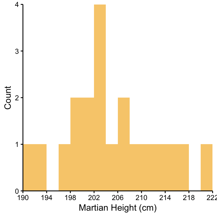
Figure 3.1: Histogram of Martian height for all individuals in our sample (n = 20).
Imagine that another observation we make is that the red–nosed Martians seem to be taller, on average, than the blue–nosed Martians. Splitting the histogram of height by nose colour produces the plot in Figure 3.2.
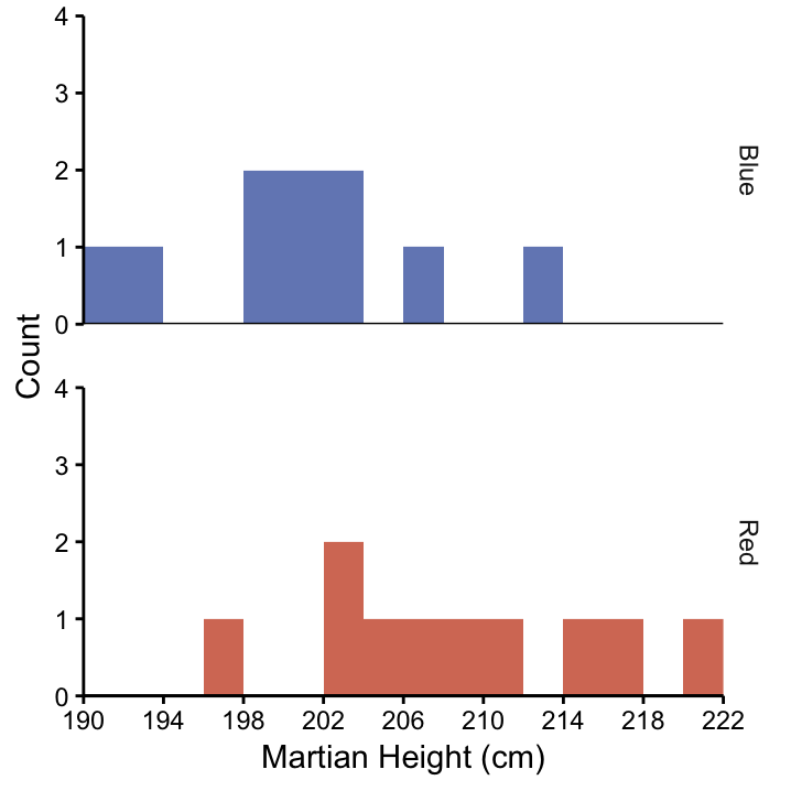
Figure 3.2: Histogram of the heights of blue–nosed and red–nosed Martians.
Based on this observation, we may generate the hypothesis that nose color has an effect on height – or the other way around. Since we’re unsure about the direction of a relationship, it’s better to talk about an association.10
Looking at Figure 3.2, we would expect that a statistical test for this hypothesis should come up with the result that nose colour and height are indeed associated. At this point we’re not ready to get into the details of the specific test appropriate for this situation, let’s just imagine that we’ve done the right test and confirmed the association.
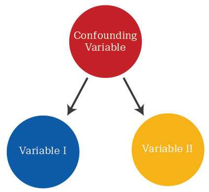
“A confounding variable alters the strength of association between two variables, that are being studied, like height and nose colour. This effect happens because the confounding variable is associated with both variables. If we want to know the real, unconfounded association between height and nose colour, we need to take the confounding variable into account when we analyse the data.”
Imagine that the next day we present our results to our team. Inspired by this interesting finding, one of the people who collected the Martians tells an anecdote of how they noticed the different nose colours for the first time. In the course of the story, it turns out that the Martians were actually collected at two different sites (let’s call them Site I and Site II). Since they noticed that there weren’t many red–nosed Martians at Site I, they were desperate to find more. They moved to Site II where many red–nosed Martians were running around but it was very hard to find blue–nosed ones.
Exercise What is the consequence of this story on the conclusion that nose colour and height are associated?
In this example, the geographic location could be a confounding variable because the red–nosed Martian histogram is dominated by Martians that lingered around in Site II while Martians from that location are under–represented in the blue–nosed Martian histogram. So perhaps height is not actually associated with nose colour, but with geographic location! There may or may not be an association between nose colour and height. Unless we use more complicated statistics where geography is incorporated in the procedure we won’t be able to distinguish between the effects of geography and nose colour, since they overlap in our data.
Exercise How could you check whether geography is a confounding variable?
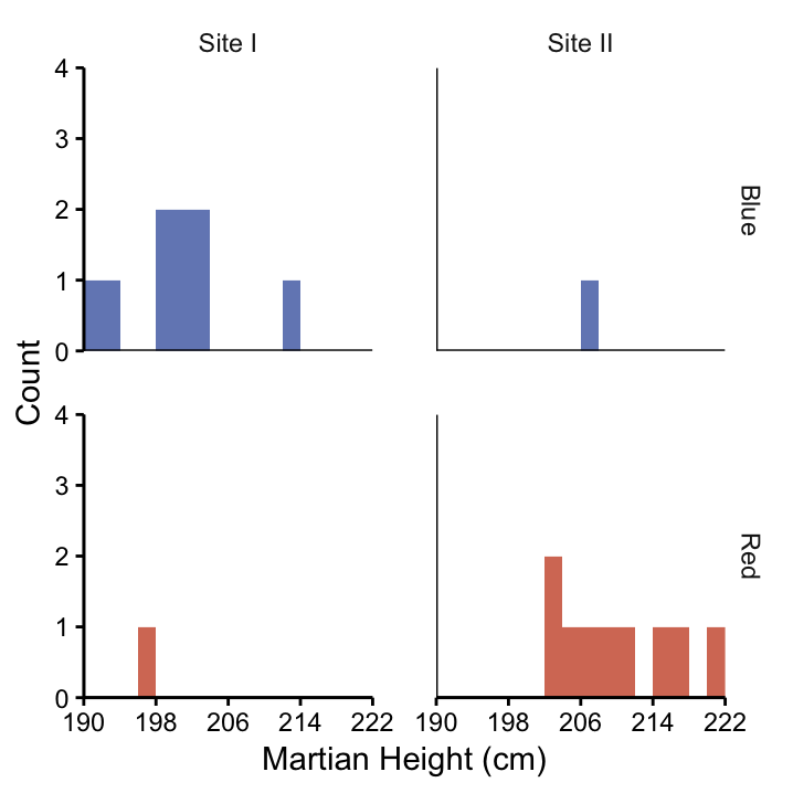
Figure 3.3: Histograms of Martian height, separated according to nose colour (rows) and location (columns). Most of the red–nosed Martians came from Site II, whereas many of the blue-nosed Martians came from Site I. Therefore, geography is a confounding variable if we want to understand the association between height and nose colour. This is a graphical way to determine if geography is a confounding variable.
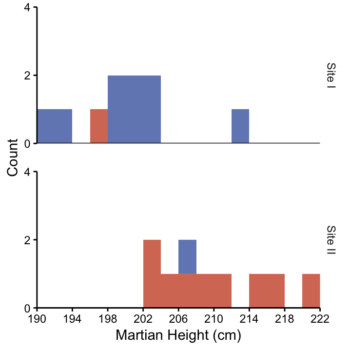
Figure 3.4: Histogram of the heights of Martians from Site I (n = 10) and Site II (n = 10).
3.5 Observational Studies vs Experimental Design
Generally speaking, there are two types of studies, observational and experimental. Especially in observational studies it’s hard to completely get rid of confounding variables, whereas you have a good shot with a well–designed experimental study. To see this, consider the situation where we’re interested in the effect of a certain treatment on some outcome. In both, observational and experimental studies the sample should contain individuals that have and those that have not received the treatment, BUT…
In observational studies, all you can do is to observe which individuals happened to have received the treatment and which haven’t. There is no way for you to influence the `treatment administration process’. Confounding variables can therefore potentially be a major issue.
Consider studying the relationship between smoking (the treatment) and lung cancer (the outcome). For your study, you’d would have to accept the smokers and non-smokers as they are since you can’t force people to smoke lots of cigarettes. Any association between smoking and lung cancer you observe in your dataset could therefore be confounded by factors that made the smokers start smoking in the first place. All you can do here is to record the potential confounding factors as variables in your dataset in addition to treatment and outcome, and to use statistical methods afterwards to account for the effect of these variables.
In experimental studies you can determine which individuals get the treatment. Here, confounding can be prevented much easier than in observational studies.
To show how this can be done, let’s return to our Martians.
Suppose we wanted to measure the Martian running time for 100 meters. We hypothesise that they could run faster if we give them the universal power food - chocolate chip cookies. To test this hypothesis an experimental design is drawn up whereby Martians are divided into two groups - one is given cookies and the other is not. As opposed to smoking, the one–off cookie treatment is easy to control and to carry out!
Now imagine that the experiment was planned in such a way that the cookie-eating group consists of all the young Martians. After measurements and statistical tests, we find that giving out cookies significantly enhances the athletic ability of our Martians. Striking!
Exercise What’s wrong with this conclusion? What would be a better way of conducting this experiment?
The benefit of being able to choose who gets the treatment in an experimental design is that you can actively avoid obvious confounding. This benefit can be maximised by randomisation which helps to turn potential confounding factors (i.e. unwanted systematic variation) into random variation that statistics is good at dealing with.
3.6 Proxy Measurements
It seems that our team of astronauts is not the best group for the statistical analysis. The troubles get worse when they try to measure Martian intelligence:
How should Martian intelligence be measured? We can’t measure it directly, since there is no measurement instrument like we had for height or time to run 100 m - we don’t even speak their language! One of the astronauts suggests to simply measure the circumference of the head, which we can measure, as a proxy for intelligence.
Exercise What are the assumptions we make when using head circumference as a proxy for intelligence? Are they justified?
Exercise What are some examples of proxy measurements you will use in your own research? What are their limitations?
Be cautious with proxy variables. Choose them wisely, and be explicitly aware of their limitations.
3.7 Generating a hypothesis
So far, we have mainly talked about problems that can occur when you generate your dataset. However, the main goal of our Martian study is to use our sample of Martians to draw conclusions about the entire Martian-kind! Although we are still in the collection part of the workshop, let’s risk a glimpse of what’s coming up.
An important part of statistics is hypothesis testing. In order to do this, we need a hypothesis.11 A hypothesis is a still-to-be-confirmed explanation of the world which we want to test using the data. But where do we get sensible hypotheses from?!
Our astronauts observed that the mean height of Martians in our entire sample is 205 cm. From this they generate the hypothesis that the mean height of the entire Martian population on Mars is 205 cm! We can write this as:
\(H_0\): \(\mu\) = 205 cm
After this brilliant idea, they then go on to test this hypothesis using the data at hand!
Exercise This is not good scientific practice! Can you think of what the problem here is?
The statistical hypothesis we test should be based on some idea we had before we collected the sample that we use to test it! In our case, this is the first time anybody has ever seen Martians so we don’t have an a priori hypothesis that we can test with the data at hand! However, that doesn’t mean our sample is useless. A careful and thorough sample description gives us a feeling for the type of data we get when we look at Martians, and is a tool for generating interesting hypotheses. Always keep in mind:
With regards to statistical hypothesis testing, there are two things we can do with a given sample: generate a hypothesis, or test a hypothesis. We can’t do both on the same dataset!
To illustrate this point a bit more, you should realise that generating and testing your hypothesis on the same sample is like choosing which team to bet on after a football game has finished. The data are bound to confirm your bet! In research, such a procedere would imply that you’re likely to obtain results that others can’t reproduce.12
At this point in our story, the astronauts are pretty disappointed, since some statisticians told them that hypothesis testing won’t work when all the knowledge about the Martian population we have is based on the single sample of 20 Martians. Although they didn’t like it, the argument that they would get results that others are unlikely to reproduce was pretty convincing. They agreed to be content with a sample description for now and generate some good hypotheses for the next trip to Mars.
3.8 Chapter Summary and Outlook
In this chapter we saw many things that can go wrong when you obtain your dataset and when you want to use it for inferring something about the entire underlying population. In essence, what makes these things so challenging is the fact that we have to cope with different sources of variation:
Systematic error, i.e. the systematic noise you get from using a biased sampling sheme or from not accounting for confounding variables. This is what you want to avoid as much as possible!
Random error, i.e. the random noise that you can’t avoid.
In this context error is also refered to as variation, so you’ll also see people refer to systematic variation and random variation.
Systematic effects caused by real relationships, i.e. the effect of interest that you want to study. In the following chapters we’ll call this the signal. This is what you can write interesting papers about!
In the light of this, we can say that we want to use statistics during the entire research process. In particular, we want to:
- Eliminate as much systematic error as we can during the collection stage. i.e. by developing a proper sampling strategy or carrying out experiments.
- Describe our sample to get an idea about the type of data we’re dealing with and to generate hypotheses.
- Quantify random error (the noise).
- Uncover underlying principles, i.e. systematic effects and relationships of interest (the signal).
- Express our level of confidence about these underlying principles, as we will see, this will be done in many cases by calculating the signal:noise ratio.
So far, we’ ha’ve discussed the first point, sample collection and its associated pit-falls. Hopefully we’ve convinced you that although it’s a lot of work, a thorough planning of your study before the data-collecting phase is worth the effort, since in the end you can be more confident about your results!
The rest of the workshop will cover points 2–5. Let’s take a break and in the next chapter we’ll continue with descriptive statistics.
Martians were collected with their written consent, of course, and full approval of the ethics commission!↩
Statisticians even kind of like random errors, since they ensure that they keep their jobs.↩
We cannot avoid errors but we need to be careful not to introduce systematic errors, statistics is very good at dealing with random errors but can potentially be thrown off by systematic errors↩
Here we set aside concerns about using the same sample to generate and test a hypothesis for the sake of the example. Keep in mind that in reality this would not be appropriate, cf. Generating a hypothesis, @ref(sub:generating_a_hypothesis).↩
Here we mean a statistical hypothesis, as we explain in the next section.↩
You can probably see why statisticians have a reputation for being the smart-assed spoiled-sports in their research institutes!↩