Chapter 5 Theoretical Probability Distributions
In the previous chapter we focused our considerations entirely on the sample that we have in front of us. However, as we mentioned earlier (see @ref{Mars}), the purpose of collecting a sample usually is to infer characterics of the underlying study polulation. In order to do so, we often utilise theoretical probability distributions that can be viewed as models that characterise study populations and that will help us when it comes to statistical inference later on.
5.1 About Distributions
Let’s go back to Figure 4.2 for a second. It depicts the distribution of Martian height within our sample. To be more specific, it depits the empirical frequency distribution of the variable height for the 10 Martians that we collected at site I. Another empirical frequency distribution of the same variable is shown in Figure 3.1. Here the Martians that we collected at site II are also included. We see that it looks slightly different but has the same basic features (it’s roughly symmetrical about the mean).19
Unfortunately, every sample is likely to result in a different empirical frequency distribution and probably none of them will exactly resemble the distribution of height in the entire Martian population. This is a shame because – in general – knowing the distribution of your variable of interest in the population you’re studying would provide answers to all questions that you may want to investigate!
To make things more complicated, even if we did have the chance to observe the entire study population (which we usually don’t), describing all features of the distribution (all bumps and other quirks) would probably be very cumbersome. So we need a way to simplify things and come up with a model that describes what we imagine the distribution of the variable to look like in the study population.
Models like this are referred to as theoretical probability distributions. Their general shape is governed by a mathematical formula that includes parameters that will determine features like location and spread. There are different prototype theoretical probability distributions, and which one you choose depends on the nature of the variable that you’re studying (cf. Section ??).
In this chapter, we’ll cover the Binomial distribution that is a model for binary variables and the Normal distribution20 that is the most common model for symmetrical continous variables.
Before we start, let’s recapitulate what we’ve learned so far:
An empirical frequency distribution is the distribution of a variable that we observe in a given sample.
A theoretical probability distribution is a mathematical model for the distribution of a variable in the study population. By picking a type of theoretical probability distribution for a variable we fix the general shape of distribution. This is like having a model of how we think the world works.
Exercise Empirical frequency distributions can either be reported in terms of absolute or relative frequencies. Which of the two would be more compatible with theoretical probability distributions?
Exercise Can you think of a property that empiricial (relative) frequency distributions and theoretical probability distributions have in common?
5.2 The Binomial Distribution
As mentioned above, the Binomial distribution is a model for the distribution of a binary variable. To explain things in this context, we’ll start with the most used and maybe also most boring example in statistics, i.e. heads or tails when tossing a coin a certain number of times – sorry about this example, bear with us for a minute!
We said that theoretical probability distributions can be seen as models of how we imagine the world to be. When we are tossing a coin, a natural view of the world’s status would be that the coin is fair, i.e. for every toss the probability for head is 0.5 – same as for tails. With this assumption, we can come up with the distribution for the number of heads that we expect when we toss the coin more than once, let’s say we toss it twice: the probability of getting two heads, \(p(\mbox{2 heads})\), is \(0.5\times0.5 = 0.25\), which is also the case for two tails, \(p(\mbox{0 heads})\). There are two ways of getting \(p(\mbox{1 head})\), either the first toss is heads or the second one is, thus \(p(\mbox{1 head}) = (0.5\times0.5) + (0.5\times0.5) = 0.25 + 0.25 = 0.5\). These probabilities are plotted on the left–hand side Figure 5.1.
Once you understand the above procedure, it’s easy to extend the consideration to more than two tosses, cf. the middle and right–hand side of Figure 5.1 that show all possible outcomes and the associated probabilities for 5 and 10 tosses of a fair coin, respectively.
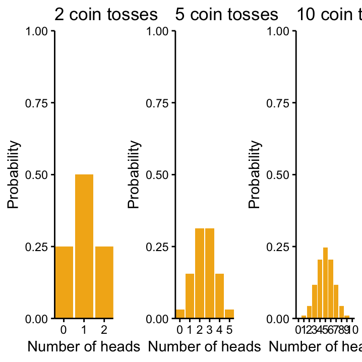
Figure 5.1: Changing n in binomial distributuions, from left to right, Bin(p = 0.5, n = 2), Bin(0.5, 5), Bin(0.5, 10).
One very cool feature of theoretical probability functions is that we can use them to probe what we image the world to look like with reality! In the coin toss example, this would mean we want to know if the assumption of a fair coin is justified. And we can do this by actually conducting the experiment and tossing the coin!
Exercise Imagine you throw the coin twice and get one head – is that fishy? What about getting only one head when throwing the coin 5 or 10 times, respectively?
At some point, we would get very suspicious about our fair coin assumption! Maybe someone tweaked it! Maybe the probability to get a head everytime you toss the coin that you are examining is actually only 0.1! Figure 5.2 shows the Binomial distribution for the number of heads that you get with this assumption for 2, 5, and 10 tosses. They seem to be much more in line with the outcome of our experiments!
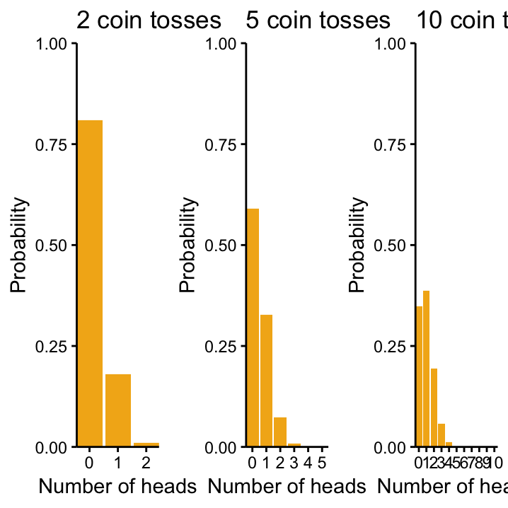
Figure 5.2: Changing p and n in binomial distributuions, from left to right, Bin(p = 0.1, n = 2), Bin(0.1, 5), Bin(0.1, 10).
Exercise If the probability of heads in a single toss is 0.1, what’s the probability of getting tails?
Now here comes the relief! Coin tosses are not the only application for Binomial probability distributions! They can be used for any binary variable that is sampled a certain number of times, e.g. a phenotype that can be present or absent in some brain cells or a disease that can be early–stage or advanced in a cohort of patients.
The generic way to deal with the Binomial distribution is to call one of the outcomes the success21 and to assign to the event “success” a certain probability, \(p(success)\), that you expect in a single trial, where “trial” can mean coin toss, individual cell or patient – depending on what you’re looking at.
With these definitions, we can make the general statement that the Binomial probability distribution is goverened by two parameters:
The number of trials \(n\) that determines the potential number of successes which can be any integer from 0 to \(n\) (look at the \(x\)–axes in Figure 5.1 and Figure 5.2).
The probability of success \(p\) that governs the shape of the distribution.
To specify a particular Binomial distribution with these two parameters, we write Bin(\(n\), \(p\)).
Use the Binomial Distribution App, explore how changing these parameters affects the probability distribution and answer the following questions:
Exercise What is the probability of finding exactly 9 heads when tossing a fair coin 25 times? What about 16 heads?
Exercise What is the probability of finding 9 or less heads when tossing a fair coin 25 times? What about 16 or more heads?
In the Martian dataset, nose colour is a binary variable that can take the two values blue and red. Let’s have a look how we can apply the Binomial distribution here!
In our sample of Martians from site I, we observed that 90% have blue noses. If this observation is a good model for the entire Martian population, we would expect the number of blue–nosed Martians to follow a Binomial distribution with \(p(blue \, \, nose) = 0.9\).
As our dataset also contains the \(n=10\) Martians that we (independently) collected at site II, we can directly probe this assumption about the state of the world: at site II, we observed 10 % blue-nosed Martians. Does this fit with the model?! Not really – we don’t even need to look at the Bin(\(10\), \(0.9\)) distribution for this!
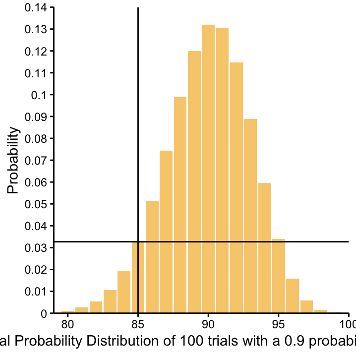
Now, consider a situation that is a bit more ambiguous. Imagine we didn’t have the site II Martians, so our hypothesis \(p(blue \, \, nose) = 0.9\) still holds next time we go to Mars. This time we collect a sample of 100 Martians. The Binomial distribution for the number of blue–nosed Martians in this sample that is in line with our hypothesis is Bin \((100, 0.9)\). It is depicted below. According to this distribution, we most likely expect to observe 90 blue-nosed Martians, i.e. 90 % of the sample. It turns out, however, that instead we observe 85. How likely is this?
Use the Binomial Distribution App to answer the following questions:
Exercise Imagine that we knew that the true \(p(blue \,\, nose)\) of getting a blue-nosed Martian is \(0.6\), what is the probability of observing \(25\) blue-nosed Martians in a sample of 30 Martians?
Exercise What is the probability of observing \(25\) or more blue-nosed Martians if the \(p(blue \,\, nose)\) is \(0.6\)?
5.3 The Normal Distribution
The Binomial distribution serves as a model for binary variables. When we are dealing with continuous variables instead, a very common model is provided by the Normal distribution22. It has the following very simple and famous equation (which you don’t need to memorise):
\[\begin{equation} f\left(k\right) = \binom{n}{k} p^k\left(1-p\right)^{n-k} \tag{5.1} \end{equation}\]
\[f(x) = \frac{1}{\sigma\sqrt{2\pi} } \; \mbox{e}^{ -\frac{(x-\mu)^2}{2\sigma^2} }.\]
\[\begin{equation} f(x) = \frac{1}{\sigma\sqrt{2\pi} } \; \mbox{e}^{ -\frac{(x-\mu)^2}{2\sigma^2} }. \tag{5.2} \end{equation}\]
To understand this formula, let’s look at the components of the right–hand side of the equation. Apart from \(x\) (which is just the argument of the function), it contains the number 2 (nothing special)23, the natural constants \(\mbox{e}\) and \(\pi\) (which are just numbers), and two Greek letters \(\mu\) and \(\sigma\) that don’t have an immediately obvious interpretation.
Just like \(n\) and \(p\) are the parameters of the Binomial distribution, Bin(\(n\), \(p\)), that control the appearance of the probability function (cf. Figures 5.1 and 5.2), \(\mu\) and \(\sigma\) are the parameters of the Normal distribution that govern the shape of the associated curve. As a short hand, we can just write \(N(\mu, \sigma^2)\). A generic example of a Normal curve is shown in Figure ??.
Let’s take note of the following properties of the curve and the role of the two parameters:
5.3.1 The parameter \(\mu\)
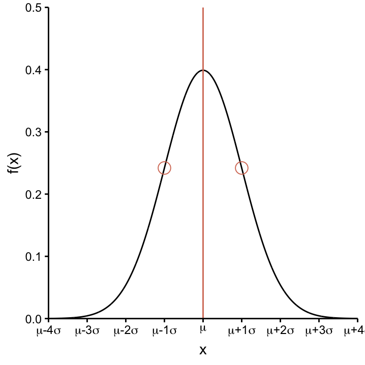
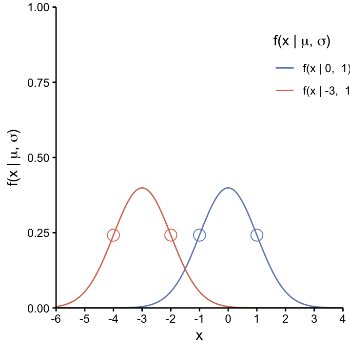
The parameter \(\mu\) dictates the location of the curve on the \(x\)–axis: the curve peaks at \(\mu\) and is decreasing in a symmetrical and monotone way as it moves away from \(\mu\). This is further demonstrated in Figure fig:conSvarU which shows two Normal distributions with different values of \(\mu\) (\(\mu=0\) and \(\mu=-3\)) while keeping \(\sigma = 1\) constant. As we will see, \(\mu\) can be interpreted as the (usually unknown) population mean of the continuous variable that we model using the Normal distribution.
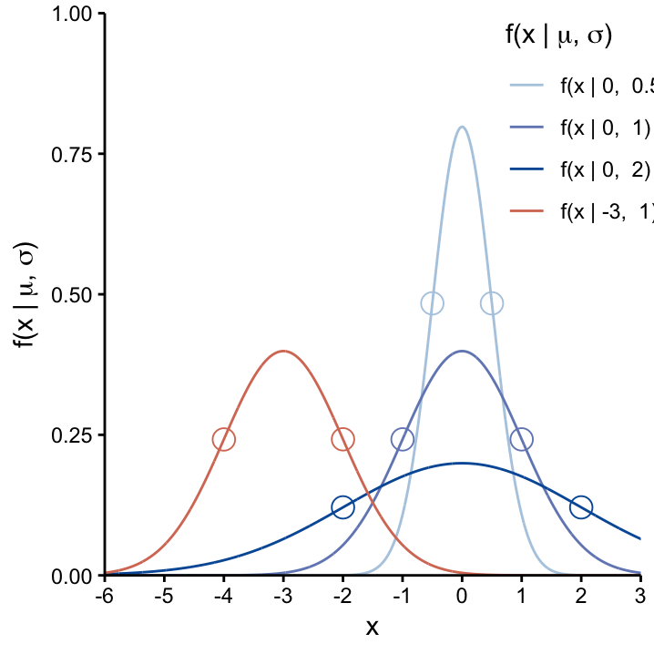
The effects of changing \(\mu\) on the Normal curve. As \(\mu\) changes, so does the center of the distribution. The width of both curves is identical, since their \(\sigma\) values are the same. The infliction points, corresponding to \(\mu\pm1\sigma\), are shown as dots on each curve.
5.3.2 The parameter \(\sigma\)
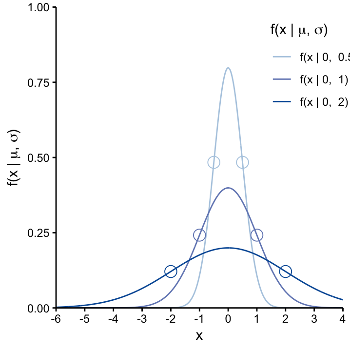
The parameter \(\sigma\) determines the width of the curve: the two infliction points are situated at \(\mu\pm1\sigma\). This is further demonstrated in Figure ?? which shows three Normal distributions with different levels of \(\sigma\) (\(\sigma=0.5\), \(\sigma=1\), \(\sigma=2\)) while keeping the center constant at \(\mu =0\). We see that the curve becomes higher and narrower as \(\sigma\) decreases and, conversly, becomes flatter and broader as \(\sigma\) increases. Thus the Normal curve is like an accordion, it can be anything between thin & tall and wide & short. As we will see, \(\sigma\) can be interpreted as the (usually unknown) population standard deviation of the continuous variable that we model using the Normal distribution.
fig cap: The effects of changing \(\sigma\) on the Normal curve. As \(\sigma\) increases (from light to dark blue curves), so does the spread of the distribution. The curves become wider and flatter whereas the height decreases. The infliction points, corresponding to \(\mu\pm1\sigma\), are shown as dots on each curve.
5.4 Normal probabilites – the area under the Normal distribution
The Normal distribution can be used as mathematical description of how we imagine a continous variable \(X\) (e.g.,\(X\) could be Martian height) to behave in the study population. It therefore has the same function as the Binomial distribution for binary variables, but there is a big difference! From the Binomial distribution, the expected probability of a certain outcome (e.g. finding 85 blue–nosed Martians in a sample of 100 Martians when \(p(blue \,\, nose) = 0.9\)) could be directly obtained but with a continous distribution this is not possible. In fact, the values on the \(y\)–axis cannot be interpreted as probabilities!
What can be interpreted as probabilities though is the area under the curve. This is because the entire area under the curve of any Normal distribution integrates to one.24 Take for example the red curve in Figure ??. While it is not possible to determine the probability for \(X=-2.5\), it easy to see that the probability for \(X< -3\) is 50% because the area under the curve to the left of \(\mu\) is just as big as the area under the curve on the other side.
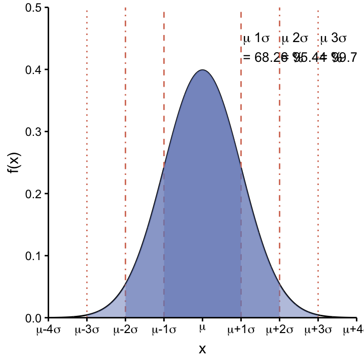
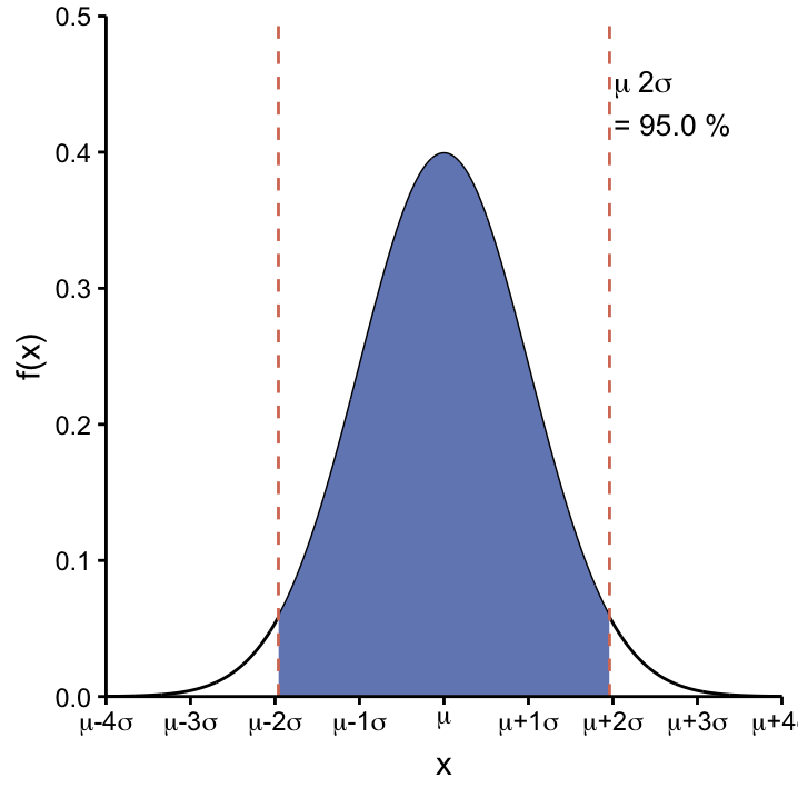
For a generic Normal distribution \(N(\mu, \sigma)\), there are a number probabilities that are easy to remember. These are the probabilities that \(X\) takes a value within certain central intervals around \(\mu\), cf. Table @ref(tab:Normal_perc). The integrations that need to be carried out to calculate the probabilities are shown in Figure ??. Notice that less than 5% of the distribution is to be found beyond \(\mu\pm2\sigma\).
| Probability | Central Interval |
|---|---|
| 68.26 % | [\(\mu-1\sigma, \mu+1\sigma\)] |
| 95.44 % | [\(\mu-2\sigma, \mu+2\sigma\)] |
| 99.72 % | [\(\mu-3\sigma, \mu+3\sigma\)] |
| ————- | ———————————— |
| 95 % | [\(\mu-1.96\sigma, \mu+1.96\sigma\)] |
figcap: Central Intervals of the Normal distribution. top: For any Normal distribution defined by \(\mu\) and \(\sigma\), 68.26% of the area under the curve will lie in the interval \([\mu-1\sigma, \mu+1\sigma]\), 95.44% in the interval \([\mu-2\sigma, \mu+2\sigma]\), and 99.72% in the interval \([-3\sigma, 3\sigma]\). bottom: 95% of the area under the curve is found within the interval \([\mu-1.96\sigma, \mu+1.96\sigma]\).
Let’s have a second look at the 95% central interval [\(\mu-1.96\sigma, \mu+1.96\sigma\)]. If we apply it to the Normal curves in Figure fig:varSconU that are centered around \(\mu =0\) we can appreciate the influence of \(\sigma\). As \(\sigma\) increases, the curves get broader and so do the 95% central intervals: [\(-0.98, 0.98\)] for \(\sigma = 0.5\), [\(-1.96, 1.96\)] for \(\sigma = 1\), and [\(-3.93, 3.92\)] for \(\sigma = 2\). If you want to remember one of them, pick the second one as it will reappear a lot later!
Use the Normal Distribution App to explore the parameters and central intervals of the Normal distribution. Also answer the exercises below!
In our Martian dataset, the continous variable that we looked at was height. As the associated empirical frequency distributions are roughly symmetrical around the mean (cf. Figures 4.2 and ??), it seems OK to use the Normal distribution as model for the variable height in the underlying population (we’ll discuss a more formal check for this in a bit, cf. Section ??).
Exercise Consider the model that the height of Martians at site I can be described by the Normal distribution of \(\mu = 200\) cm and \(\sigma = 6\) cm. 95 % of Martians at site I fall into what interval?
Exercise Now, consider that the model that the height of Martians at site II can be described by the Normal distribution with a \(\mu = 210\) cm and \(\sigma = 1\) cm. 95 % of Martians at site II fall into what interval?
Exercise Make a sketch of the two Normal distributions on a common scale in the space provided:
Exercise Imagine that we are presented with a \(215\) cm tall Martian. Draw a vertical line on your plot from the previous exercise.
Exercise Given our assumptions about the distributions of Martian height at site I and II, which site do you think this Martian came from, and why?
5.5 Z-scores and the Standard Normal Curve
Notice that in the exercise above, we had to draw two Normal curves and then position our mystery \(215\) cm tall Martian in this landscape to compare the likelihood of the two scenarios (sites). Luckily there is an easier way to make this comparison by standardising the value of unknown origin (\(215\) cm in our case) against our two models under consideration. That is the role of Z–scores:
Z–scores allow us to normalise disparate data onto a common scale!
The Z–score for any given value \(X_i\) with respect to a model that assumes a mean value of \(\mu\) and a standard deviation of \(\sigma\) can be obtained using the following normalisation:25
\[Z_i = \frac{X_i - \mu}{\sigma}.\]
We’ll encounter this surprisingly simple yet useful equation many times throughout the workshop! Here we’ll demonstrate its value by re–addressing the exercise above.
Exercise Consider the population described by \(\mu = 200\) cm and \(\sigma = 6\) cm, complete the following table:
| \(x_i (cm)\) | 182 | 188 | 194 | 200 | 206 | 212 | 218 |
|---|---|---|---|---|---|---|---|
| \(x_i - \mu\) | |||||||
| \(z_i\) |
Exercise Continuing with the population described by \(\mu = 210\) cm and \(\sigma = 1\) cm, complete the following table:
| \(x_i (cm)\) | 207 | 208 | 209 | 210 | 211 | 212 | 213 |
|---|---|---|---|---|---|---|---|
| \(x_i - \mu\) | |||||||
| \(z_i\) |
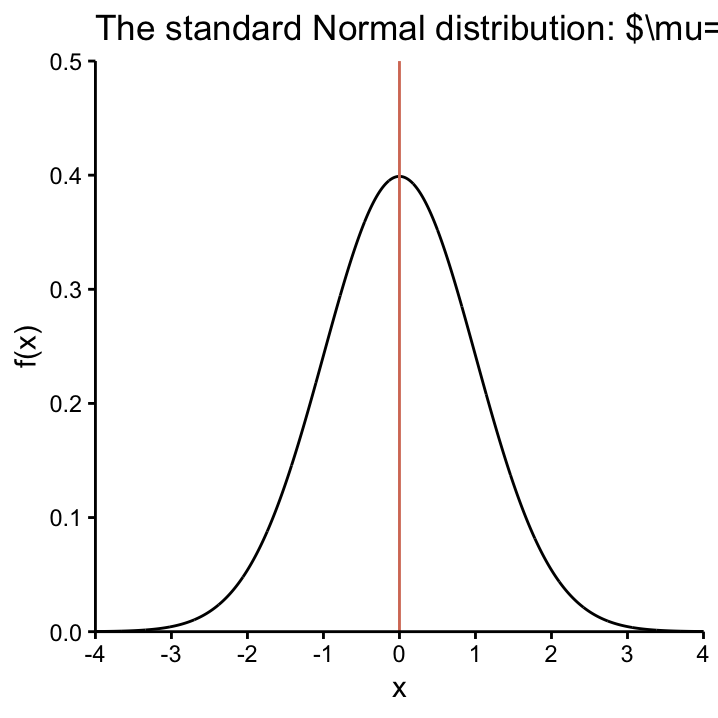
From the results of these exercises we can understand that Z–scores simply tell us how many standard deviations a value is away from the mean with respect to a given model. If the model is described by the Normal distribution, Z–scores have the very cool feature that they themselves are Normally distributed!! As they are normalised, the corresponding Normal distribution has a mean of 0 and a standard deviation of 1. This all follows logically from the equation for Z–scores and can be written in a shorthand form as:
\[Z_i = \frac{X_i - \mu}{\sigma} \sim N(0, 1).\]
The distribution \(N(0, 1)\) is called the standard Normal distribution and is shown is Figure StdNorm.
figcap: The standard Normal distribution is a Normal distribution with \(\mu=0\) and \(\sigma=1\), \(N(0,1)\) for short.
Why is this of any use to us? It enables us to immediately judge how unusual a value is with respect to a given model. Recall that 95% of values of any Normal curve fall in the interval \([\mu-1.96\sigma, \mu+1.96\sigma]\). In the context of Z–scores where \(\mu=0\) and \(\sigma=1\) this interval becomes \([-1.96, 1.96]\) and we immediately know that any Z–score outside of this interval is quite an unusal value! In general, the larger the absolute value of a Z–score (the further away it is from 0), the more extreme the underlying \(X\)–value is with repect to the model that is used for the normalisation.27
Exercise Returning to the mystery 215 cm tall Martian from the previous exercise. Calcuate it’s Z–scores with respect to our two models from site I and site II. Which site do you think the Martian came from, and why?
Note that you could even plot both Z–scores (e.g. as vertical lines) on the standard Normal curve. By definition they are on the same scale!
“The term empirical was originally used to refer to certain ancient Greek practitioners of medicine who rejected adherence to the dogmatic doctrines of the day, preferring instead to rely on the observation of phenomena as perceived in experience.” Wikipedia, The Free Encyclopedia, s.v. “Empirical Research,” (accessed Januar 07, 2018),
https://en.wikipedia.org/wiki/ Empirical\_Research.↩Later on we’ll also cover the \(t\)–, the \(F\)– and the \(\chi^2\)–distributions in this workshop.↩
Don’t let the term success confuse you. Which of the two outcomes you choose as the success is arbitrary! As you have only two outcomes, we automatically know that the probability of no success is \(1 - p(success)\) in a single trial.↩
The equation for the Normal distribution was developed by Karl Friedrich Gauss in 1809.↩
In Statistics the convention is that Roman letters, e.g. \(\bar{x}\) and \(s\), are used to refer to the sample, Greek letters, e.g. \(\mu\) and \(\sigma\), refer to the population.↩
Integrating to find the area under the curve for continous distributions is equivalent to summing up the individual probabilities of all different outcomes of a discrete variable.↩
In reality we don’t know \(\mu\) and \(\sigma\) so we just use \(\bar{x}\) and \(s\). We’ll come back to this point when we encounter estimation.↩
We can also understand Z–scores as \[\frac{X_i - \mu}{\sigma} = \frac{\mbox{signal}}{\mbox{noise}}.\] The signal is the systematic variation we are interested in and the noise is the random error which we cannot avoid. Keep this in mind and we’ll get back to it in the context of hypothesis testing.↩
Also note that Z–scores don’t require a unit! When you calculate them, the unit appears in both the numerator and the denominator and cancels out.↩