Chapter 10 Linear Regression - Comparing two Continuous Variables

10.1 Part 1 – Linear Models and t–tests

Now we turn our attention to the situation where we want to describe a continuous variable by another continuous variable. For this purpose, we turn to linear regression. In principle, the aim of linear regression is the same as what we covered in the previous chapters where we were investigating if knowing the level of a categorical variable helps us to predict the value of a continuous variable (two–sample $t$–test) or another categorical variable ($\chi^2$–test). With linear regression, we want to understand how well the values of one continuous variable $Y$ are explained by the values of another continuous variable $X$. As we will see, this topic is also related to the well–known concept of correlation.

A word of warning before we get started: as with any statistical technique, the calculations in linear regression can be done whenever the variables of interest fulfill the requirement, i.e. here we can compare any two continuous variables. The technique itself doesn’t care about the meaning of the variables we put into our equations⁶⁷. Biologically interesting or sensible are a different story, so even when you understand the statistical technique you’re using very well, unfortunately that’s still no excuse to switch off your brain! Although you obviously need to know the technique very well before you are able to interpret its output, it’s the interpretation of the output that’s the challenging thing, not producing it.

10.2 Linear Regression in a Nutshell

For the moment, let’s not worry about assumptions or Martians - we’ll begin with a very simple example where a single variable $Y$ has been observed on four individuals, i.e. we have four observations $y_1 = 2$, $y_2 = 5$, $y_3 = 4$ and $y_4 = 7$, cf. Figure SingleVarOLS. With the four observations, the simplest thing we can do is use the mean $\bar{y}$ (the red line in Figure SingleVarOLS) to describe this sample. Also, and this is an important point, if you were to predict the value of $Y$ of a new observation, $\bar{y}$ is the value to go for in the absence of further information.

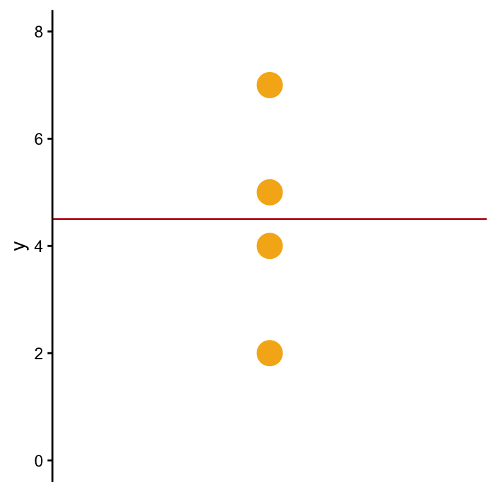
SingleVarOLS The best prediction for a single variable, $Y$, is the mean, $\bar{y}$ (red line) if not further information is available.

As a next step we’re interested to know how (and optimally also why) $Y$ varies between different individuals. Maybe the values of $Y$ come as a consequence of some other variable $X$? What we’re asking is: Can we use a second variable, $X$, to better describe $Y$? For this purpose we go back and measure the second variable. Our four observations therefore now come in pairs $(x_1, y_1)$, $(x_2, y_2)$, $(x_3, y_3)$, $(x_4, y_4)$ which are shown in Figure ??. We can still describe $Y$ using $\bar{y}$ as shown by the horizontal line, but this obviously ignores any input from the second variable. So although it’s not meaningless - we can do better than that!

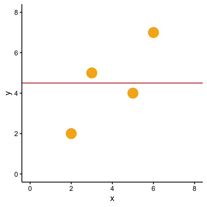
Does adding a variable X improve our understanding of Y? That is, is $\bar{y}$ still the best model for $Y$?

Compare Figures ?? and OLSYX. You’ll agree that the diagonal line drawn represents our data better than the simple horizontal line. So, if you were to predict the $Y$–value of a new observation, you’d now be eager to know the corresponding $X$–value! As a next step we want to quantify the newly discovered relationship between $X$ and $Y$ so that we are then able to make these predictions. The method we employ for this is called Ordinary Least Squares (OLS) which is a fancy term for linear regression. Among other things, OLS tells us how to find the best line: we’re looking for the line with the least squares. The least squares of what? A sensible thing to minimise and find the least squares of are the residuals, which are a very important concept in OLS:

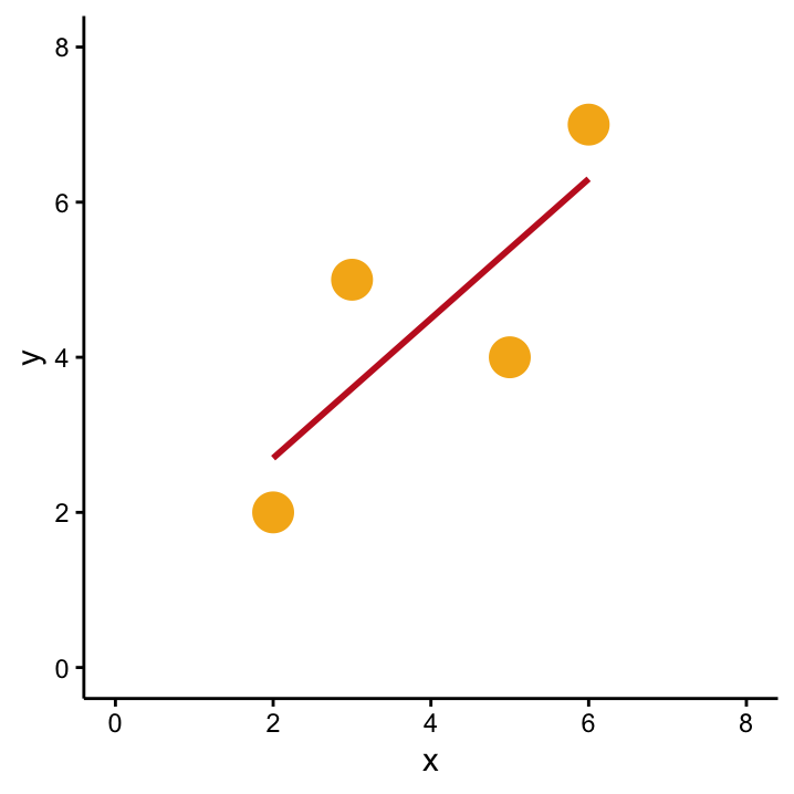An OLS model for $X$ and $Y$ describes the influence of $X$ on $Y$.

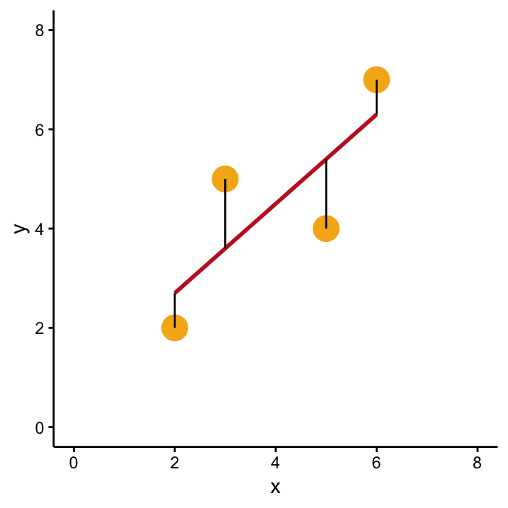The goodness-of-fit for the OLS model can be described by it’s residuals, shown in black. The sum of the squared residuals summarises this information in a single parameter.

Residuals are the (vertical) distance between each data point and the model which describes the data set.

In Figure ??, the black lines show the residuals between each data-point and the OLS model which is used to quantify the observed relation between our two variables, and the fact that we’re looking at the OLS model tells us that the drawn line is the line that results in the smallest sum of the squared residuals. This sum is commonly denoted as $SSR$ and is the criterion that is optimised in OLS.

Let’s have a look at the $SSR$ criterion to see what it’s all about: \[SSR = \sum_{i=1}^n (y_i - f(x_i))^2,\] where $f(x_i)$ is the value of $Y$ predicted from the line when $X=x_i$. The predicted value of $Y$ of a given data-point that has an $X$-value of $x_i$ is often denoted by $\hat y_i$ so that the above formula becomes \[SSR = \sum_{i=1}^n (y_i - \hat y_i)^2.\] This should look very familiar to you, because it’s basically the same thing as the sample variance of our $y$–values⁶⁸

\[s_y^{2}=\frac{\sum_{i=1}^{n}(y_{i}-\bar{y})^{2}}{n-1}\] except, $SSR$ is not scaled by $n-1$. \

So we learned that OLS finds the line $f(X)$ that most reduces the $SSR$. But can we quantify this line? It must depend on the observed data somehow – but how?! Before we give the answer to this burning question, let’s go back in time a bit and recall from some grey day in school that every line can be described by two numbers, the slope and the intercept.

The slope describes the steepness of a line. It is formally defined as the change in $f(X)$ on the $y$–axis when you go from a value $X$ to $X+1$.

The intercept is the value on the $y$–axis you get when $X=0$, i.e. when the line crosses the $y$–axis.

When we want to find the line that minimises $SSR$, we need to find the best slope/intercept combination. But how do we find it? This is the first of our burning questions that we are about to answer here. The second is whether the OLS line is really all that much better than the horizontal line drawn in Figure SimpleYX. And lastly, you may suspect already that the correlation between $X$ and $Y$ will play an important role for answering the questions. So at the end of the chapter, we will make the connection between OLS and correlation! In summary, the questions that dictate the flow of this chapter are

What is $f(X)$? That is, for each value of $X$, what is the associated value of $Y$? This is equivalent to asking about the best slope and intercept.
Is there a statistically significant relationship between $X$ and $Y$? Is the slope statistically different from zero? What is the $p$–value?
What does all of this have to do with correlation?

10.3 What is the $f(x)$?

As we mentioned above, a straight line is described by the equation \[ f(X) = \beta_0 + \beta_1 X,\]

where $\beta_0$ is the intercept⁶⁹ and $\beta_1$ is the slope of the line. In our example, we have four $X$–values, namely $x_1 = 2$, $x_2 = 3$, $x_3 = 5$, and $x_4, = 6$. So the the value on the line that correspond to $x_i$ can be written as $f(x_i) = \beta_0 + \beta_1 x_i$, where $i$ can be either 1,2,3 or 4.

As we said, OLS tells us how to get the values for the intercept and slope that produce the best fitting line for our data. Actually, the formula for the best slope is very simple and can be used with only pen and paper! It’s just two numbers divided by one another \[ \hat \beta_1 = \frac{COV(x,y)}{s^2_x} ,\] where $s^2_x$ denotes the sample variance of $X$. But what about the numerator? This is a thing called covariance which is defined as:

\[COV(x,y) = \frac{\sum_{i=1}^{n}(x_i-\bar{x})(y_i-\bar{y})}{n-1}. \]

Exercise In our example, $x = $ 2, 3, 5, 6, ($\bar{x}=$ 4, $s^2_x=$ 3.33 ) and $y=$ 2, 5, 4, 7 ($\bar{y}=$ 4.5, $s^2_y=$ 4.33). Using the formula above, calculate $COV(x,y)$!\

Now that we know $COV(x,y)$ we can calculate the optimal slope as $\hat \beta_1 = COV(x,y)/s^2_x = 3/3.33 = 0.9$.

Easy, but what about the intercept?!⁷⁰ Well, if we have the slope of the our optimal line, the formula for the intercept is even easier, namely \[ \hat \beta_0 = \bar y - \hat \beta_1 \bar x\] which in our example is $\hat\beta_0 = 4.5 - 0.9 \cdot 4 = 0.9$.

The equation of the line that optimally fits the data in our example is therefore \[\hat f(X) = 0.9 + 0.9 X\] which means that if we want to predict the $Y$–value for an observation with an $X$–value of $x_i$, we’d get \[\hat y_i = 0.9 + 0.9 x_i.\]

So far so good, but as we heard many times, there’s uncertainty that we need to account for! The four data points that we used for calculating intercept and slope are actually only a sample from a bigger population. To make things worse, they are not even a very big sample. So $\hat \beta_0$ and $\hat \beta_1$ are probably not equal to the underlying true population values that belong to the line which really describes the relationship between $X$ and $Y$ in the entire population. They are only estimates! In case you have been wondering, this is the reason why we put the little hats on top of them.

The values $\hat \beta_0$ and $\hat \beta_1$ are estimates for the underlying population intercept $\beta_0$ and slope $\beta_1$. There is uncertainty attached to them!

Usually, we are particularly interested in the uncertainty associated with $\hat \beta_1$. Could it be so big that despite the fact that our estimate from the sample is $\hat \beta_1 = 0.9$, the true underlying population slope is $\beta_1=0$?! This is the next question we’ll look at?

Exercise What would it mean if $\beta_1=0$? Use the figures at the beginning of this section!

10.4 Hypothesis testing in linear regression

As we saw, in linear regression we are interested in the question whether our estimated coefficient $\hat \beta_1$ is statistically different from zero. So we are back in the framework of hypothesis testing where we need a null and an alternative hypothesis.

Exercise What are suitable null and alternative hypotheses?

Put in words, the null hypothesis means that the second variable, $X$ does not help us to explain or predict the values of $Y$. This is like saying that we might as well have used the sample mean $\bar{y}$ as a predictor, because the addition of the second variable didn’t add any information. This is the situation we saw in Figure ??.

Good news, guys! Despite the fact that we’re currently exploring different questions than before, the principles that you learned so far stay the same! Although we are talking about a slope and not mean values, the test problem \[ H_0: \beta_1 = 0 \quad \quad \mbox{versus} \quad \quad H_1: \beta_1 \neq 0,\] can be dealt with using a one–sample $t$–test⁷¹. We know how it goes from what we learned in the previous chapter, but let’s spell it out in detail. As usual, we need a test statistic of the form

\[ \frac{\mbox{signal}}{\mbox{noise}} = \frac{\mbox{(observed value - hypothesised value)} }{\mbox{scale factor}}. \]

The different components are:

observed value: The observed value is the best slope we calculated from the observed data, i.e. $\hat \beta_1$.
hypothesised value: The null hypothesis is that the true slope is equal to zero!
scale factor: In the one–sample $t$–test, the scale factor was the $SEM$ which is the standard deviation of the estimate $\bar x$. Here we need the standard deviation of the estimate $\hat \beta_1$, which we’ll call $sd(\hat \beta_1)$. To keep things simple, we won’t get into the details of how this is calculated. Just realise that it’s the same concept we saw before.

With the information above, we see that the test statistic that we are looking at has the form \[ \frac{\hat \beta_1 - 0}{sd(\hat \beta_1)} = \frac{\hat \beta_1}{sd(\hat \beta_1)}.\] As usual, we need to compare the value we observe for this statistic with a null distribution which in this case is the $t$–distribution with $n-2$ degrees of freedom. So we can write⁷²

\[ \frac{\hat \beta_1}{sd(\hat \beta_1)} \stackrel{H_0}{\sim} t_{n-2}.\]

Like in the all the other tests, we have to see where the observed value of our test statistic sits on the null distribution. If it’s far from zero, we get a small $p$–value and it’s unlikely that $H_0$ is true. By the way, if you want to test whether the intercept is statistically different from zero, everything is the same. You can just replace $\hat \beta_1$ with $\hat \beta_0$.

Table: ?? contains the computer output we get for our little example:

Output for simple linear regression from our example. Note that the second row corresponds to the slope. It is denoted with ‘x’ because the slope corresponds to the influence of $X$ on $Y$.
	Estimate	Std. Error	t value	Pr(>\|t\|)
(Intercept)	0.9000	2.1290	0.42	0.7136
x	0.9000	0.4950	1.82	0.2106

Exercise Can you interpret all the numbers in Table ???

Exercise Why is the $p$–value so large although the fit of the regression line looks nice?

One of the things you need to be aware of when you interpret the output of linear regression & co: correlation does not equal causation!↩
If you don’t remember why the values are squared in $s^2$, refer back to page . The residuals are squared for the same reason. Also note that $s^2_y$ is the (unnormalised) $SSR$ if the second variable $X$ is ignored and the horizontal line is used!!↩
From this equation you can see that $\beta_0$ is the value you get when $X=0$, also when you move from $X=0$ to $X=1$, your $Y$–values will change from $\beta_0$ to ($\beta_0 + \beta_1$), i.e. the change is exactly $\beta_1$. This holds for any value of $X$ and $X+1$, try it!↩
Here we plug in the values for $\bar{x}$ and $\bar{y}$, which our line will pass through.↩
The underlying assumption of Normality that we need to check in the $t$–test context refers to the residuals in linear regression as well.↩
The reason why we now have $n-2$ degrees of freedom has to do with the fact that we are now estimating two coefficients $\hat \beta_0$ and $\hat \beta_1$ from the same sample of $n$ observation. This is like the situation in the two–sample $t$–test when we had to estimate the mean value of both groups.↩

Statistical Literacy

Chapter 10 Linear Regression - Comparing two Continuous Variables

10.1 Part 1 – Linear Models and t–tests

10.2 Linear Regression in a Nutshell

10.3 What is the \(f(x)\)?

10.4 Hypothesis testing in linear regression