Chapter 6 Estimation – dealing with uncertainty!
So far, we’ve discussed samples, in the context of descriptive statistics, and populations, in the context of probability distributions. The major challenge in Statistics is to connect these two parts together. That is, given what we know about the sample, what can we say about the population? This is the subject of statistical inference:
Statistical inference is the process of drawing conclusions about populations, or scientific truths, from sample data.
Why is this such a challenge? Simply put, the crux of the whole matter is that the sample is usually much smaller than the population. This means that it doesn’t contain all the information available in the population. Any conclusions drawn from the sample will probably not exactly hold for the entire population so it is important to keep in mind the following two questions:
How confident can I be that the results I got from my sample can be generalised to the population, i.e. how much noise do I have in my sample?
In case I see an interesting effect, is it real (due to some systematic pattern) or just due to chance, i.e. is there a real signal among the noise?
These two questions relate to the two major topics of inferential statistics: estimation and hypothesis testing. In estimation we measure the noise inherent in our sample, and in hypothesis testing we compare the noise to the signal by means of a signal:noise ratio.
6.1 Estimation in a nutshell
We’ll return to our Martian dataset to explain the general concept of estimation. The histogram of our 10 site I Martian heights has a shape that seems to be compatible with a Normal distribution. If we want to formalise this assumption, we’d write
\[ X \sim N(\mu, \sigma^2),\]
where \(X\) is the variable in our population, i.e. ‘height’, and ‘\(\sim N(\mu, \sigma^2)\)’ means that we assume a Normal distribution with mean \(\mu\) and variance \(\sigma^2\).
As we saw in Chapter cha:understandingprobability, once we accept the model of a Normal distribution, \(\mu\) and \(\sigma^2\) are the only unknown features of the height in our Martians population. Unfortunately, we don’t know \(\mu\) and \(\sigma^2\) and all the information we have is contained in our sample
It seems we have to accept the fact there is no way for us to know the exact population parameters, so we need to use our sample to get a rough idea about their values. For example, we could use the known sample mean of the Martian height (\(\bar{x} = 200\) cm) instead of the unknown population mean \(\mu\) for any further statements.
When we do this, the mean \(\bar{x}\) is not only a descriptive statistic for the location of our sample, but now it’s also an estimate of the unknown population mean \(\mu\). While this seems to be obvious and only a matter of wording, it actually has some interesting conceptual implications! Once we realise that the sample that gives rise to our value \(\bar{x}\) was drawn randomly and that another sample would probably have resulted in a different value, we really would like to answer 3 important questions:
Q1: Is there a systematic error in using \(\bar{X}\) instead of \(\mu\)? i.e. Is \(\bar{X}\) an unbiased estimator of \(\mu\)?
Q2: How variable is \(\bar{X}\)? Q2: i.e. How much does \(\bar{X}\) depend on our given sample? How much would it vary if we had, by chance, taken a different sample from the same population?
Q3: Is \(\bar{X}\) the best estimator of \(\mu\)? i.e. Is there some other location statistic that has better properties than \(\bar{X}\), with respect to Q1 and Q2?
These questions are what estimation is all about! Estimation is about knowing the properties of the descriptive statistics we calculate from the sample when we use them to infer population characterisics. In particular we want to assess the uncertainty that is associated with the conclusions obtained from the data at hand. This in turn helps us to judge the reliability of our findings!
To answer the above questions there is an important concept we have to understand. If you learn only one thing from this workshop, then let it be that
6.2 Descriptive statistics have distributions in inference!
Descriptive statistics have distributions!? Let’s use a simulation to see what we mean: assume that the Martian height in our population does follow a Normal distribution with \(\mu=200\) cm and \(\sigma=6\) cm.28 Now imagine that instead of our single sample we could take many samples, \(m\) say, and that for each sample we calculate the sample mean such that we’d have \(m\) sample means: \(\bar{x}_1, \bar{x}_2, \ldots, \bar{x}_m\).
Video: What happens when we take multiple, independent simple random samples from the same population?
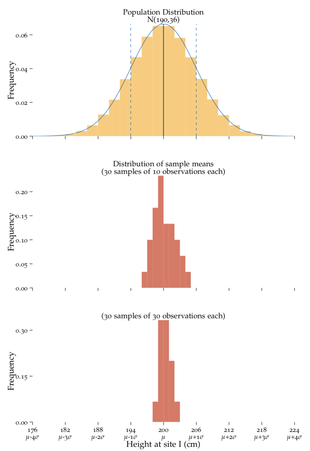
Figure 6.1: Large sample sizes.
Taking 30 random samples from a population with known parameters. top: The population distribution. We generated a population with a known mean of \(200.00\)cm and a standard deviation of \(6.00\)cm. middle: The distribution of 30 sample means taken from this population, each containing 10 observations. bottom: The distribution of 30 sample means taken from this population, each containing 30 observations. In both the middle (\(n=10\)) and bottom (\(n=30\)) plots, the mean of the sample means is centered on the original population mean. A higher \(n\) results in a narrower distribution of sample means (bottom) compared to smaller \(n\) values (middle).
Each time we draw a sample we observe a different \(\bar{x}\)! E.g. a sample that by chance contains the tallest Martians will probably provide a much higher \(\bar{x}\) than a sample that by chance contains the shortest Martians. What does this mean? To use a bit of theoretical Stats jargon, you just saw that.
The sample mean is a random variable that has a distribution!!!
So when you want to use the sample mean \(\bar X\) to infer the unknown population mean \(\mu\) it’s the properties of this random variable that we are interested in. Although it may sound strange at first, this is actually the intellectual quantum leap you’ll have to manage when you want to understand inferential statistics. The rest will fall into place from this! As this is such an important point, so let’s paraphrase what we mean here:
Just as height, \(X\), is a random variable that takes different values \(x_1\), \(x_2\), \(\ldots\) in your sample, the sample mean, \(\bar{X}\), is a random variable for which you can observe different values \(\bar{x}_1\), \(\bar{x}_2\), \(\ldots\) once the sample of Martians is drawn from the population.29
With these new insights under our belt, we are now equipped to start talking about uncertainty! Let’s tackle the three questions we presented on page EstimQuest!
6.3 Q1: Is there systematic error?
Although in reality we usually only have a single sample to draw conclusions from, we just saw that our \(\bar{x}\) is just one of many \(\bar{x}\) values we could have obtained. Nonetheless, we’re still going to use this as an estimate of the underlying population mean \(\mu\). From the video and Figure 6.1, we also learned that our single \(\bar{x}\) is drawn from a distribution of \(\bar{X}\), so in order to answer our three questions in ??, let’s describe the shape of the distribution.
Exercise After watching the video, and studying Figure 6.1, how would you describe the distribution of the sample means?
The distribution of \(\bar{X}\) is centered around the population mean \(\mu\), so although the individual values \(\bar{x}_1\), \(\bar{x}_2\), \(\ldots\) are usually not exactly equal to \(\mu\), the results are fine on average. In other words, the sample mean \(\bar{X}\) is an unbiased estimator for the underlying population mean which can be written as
\[\mu_{\bar{X}} = \mu,\]
where \(\mu_{\bar{X}}\) denotes the mean of the distribution of the sample mean \(\bar{X}\). This is actually a very desirable property because it means that we do not make a systematic error when we use the mean of our particular sample as an estimate of \(\mu\).
6.4 Q2: The variance
It’s very good to know that there’s no systematic error in using \(\bar{X}\), but we have seen that the particular values we get from different samples vary quite a bit. It would therefore be good to quantify this variation since it determines the precision of the sample mean as an estimator for \(\mu\).
Exercise Which factors do you think influence the variance of the \(\bar{X}\)?
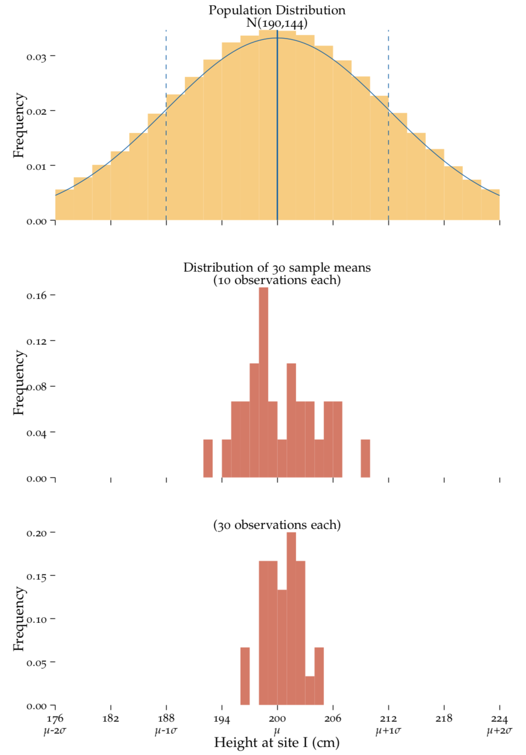
Figure 6.2: Large sample sizes.
Taking 30 random samples from a population with known parameters. top: The population distribution. We generated a population with a known mean of \(200.00\)cm and a standard deviation of \(12.00\)cm, twice as that used in Figure 6.1. middle: The distribution of 30 sample means taken from this population, each containing 10 observations. bottom: The distribution of 30 sample means taken from this population, each containing 30 observations. As in Figure 6.1, the sample means \(\bar{X}\)are centered on the population mean \(\mu\) and a larger \(n\) results in a narrower \(\sigma^2_{\bar{X}}\). However in addition to what we have already observed, here we notice that the larger population variance \(\sigma\) causes \(\sigma^2_{\bar{X}}\) to also be larger than in Figure 6.1.
Video How does the sample size influence the distribution of the sample mean?
Video How does the population variance influence the distribution of the sample mean?
From this, we can see that there are two factors, the sample size, \(n\), and the population variance, \(\sigma^2\), that influence the variance of \(\bar{X}\) that we denote as \(\sigma^2_{\bar{X}}\). This can be quantified nicely as \[ \sigma^2_{\bar{X}} = \frac{\sigma^2}{n},\] where \(\sigma^2\) denotes the variance of the population, and \(n\) denotes the sample size. This formula tells us two things
- As the variance of the population increases, so does the numerator and thus \(\sigma^2_{\bar{X}}\) gets larger.
- As the30 sample size increases, so does the denominator and thus \(\sigma^2_{\bar{X}}\) gets smaller.
What does this mean for us? The fact that \(\sigma^2_{\bar{X}}\) is influenced by the sample size is good news for us, because while we can’t do anything about the variance in the population itself31, we do usually have control over the sample size! Thus, if we want our sample mean to be a more precise estimate of the population mean we can take a larger sample.
When you think about it, this actually makes a lot of sense. The bigger the sample size, the more information about the population is being compressed into the mean. Just like in any other context, the more information you have at hand, the better the prediction will be. This is summarised in Figure 6.3.

Figure 6.3: Comparing different types of error bars.
The precision of sample means, i.e. the precision with which we can estimate \(\mu\), is inversely proportional to the underlying population variance and proportional to the sample size. Regardless of the underlying population variance, which we cannot control, larger sample sizes are always preferred.
6.5 Q3: What’s the best estimator of \(\mu\)?
By now we have seen that there are two requirements for a good estimator: being unbiased and having a small variance (i.e. high precision). The really good estimators combine both of these proporties,32 and the estimator, that combines these two requirements in the optimal way is called the minimum-variance unbiased estimator! As you might have guessed, \(\bar X\) is the minimum-variance unbiased estimator for \(\mu\). ` Let’s see what this means: while it may seem obvious to use \(\bar{X}\) as estimator for \(\mu\) we’re not restricted to that. We could have chosen any measurement of the sample to act as an estimator, e.g. we could have chosen the first value in the sample – regardless of the sample size.33 Or, if we were really stubborn, we could even have used a fixed value, 3 say, regardless of the actual sample.
Figure 6.4 shows the performance of these three estimators in the context of a bull’s eye target for shooting practice. The entire target corresponds to the values in our population and the bull’s eye is the true population mean \(\mu\). The goal is to hit the bull’s eye when we take a shot, i.e. draw a sample and calculate the estimate.
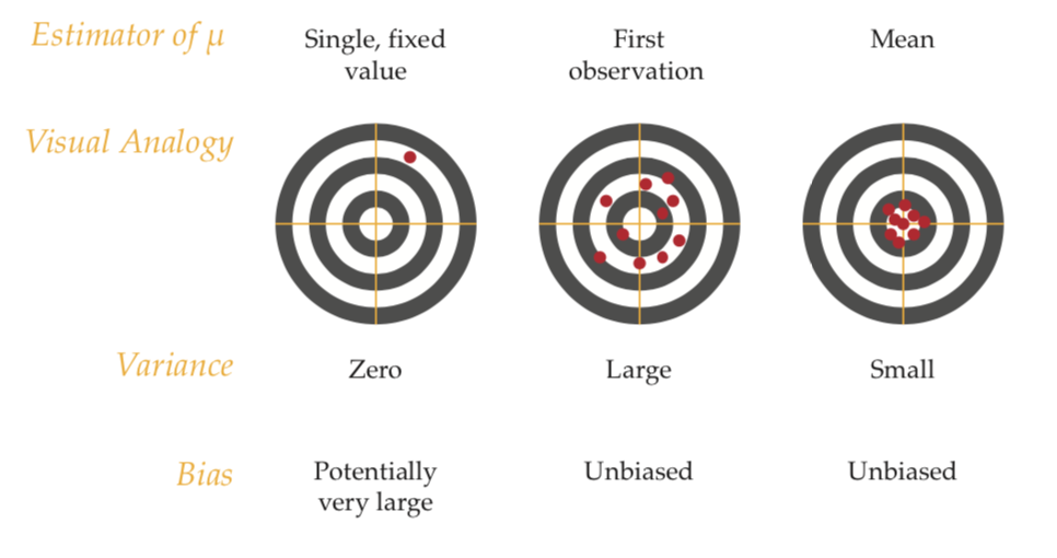
Figure 6.4: Comparing different types of error bars.
The bull’s eye analogy to understand the miniumum-variance unbiased estimator. Of all the unbiased estimators that we could have chosen, it turns out that \(\bar{X}\) has the smallest variance.
In the first scenario we fix the estimator to a specific value. Here, our variance will be zero, because no matter what the sample is, our estimator will always be the same. On the one hand, this is fantastic! We like a tiny variance. However, our estimator is likely to be very biased. It doesn’t contain any information from the sample!
In the second scenario we take the first observation of the sample to be the estimator. This has a higher variance than the fixed-number, but despite this we prefer this estimator over the fixed value because it is unbiased. As we learned this means that if we take many samples, we get it right on average.
In the third scenario we take \(\bar{X}\) as the estimator. Here, we can observe that the variance is lower then in the second scenario, and it is still an unbiased estimator. This is the ideal situation, we’ve found a balance between have very small variance and being unbiases.
Recall that Roman letters refer to the sample - \(\bar{x}\) is the sample mean - and Greek letters refer to the population - \(\mu\) is the population mean.↩
You may be wondering about the meaning behind upper and lower-case letters. The random variable \(\bar{X}\) is called an estimator whereas the individual values it takes once your sample is observed are called the estimates. The estimates are fixed values and are denoted with small letters whereas random variables are commonly denoted with capital letters. This is important if you write about statistics, but we won’t get hung up on this here.↩
The precision of the sample mean increases with the sample size!↩
If the population variance is large, we’ll always have a difficult job inferring something about the population from our sample.↩
When choosing a descriptive statistic to infer something about your population, consider if these requirements have been fulfilled. Many measurements have become standard because they do!↩
We could have also chosen to take the median, or possibly the mid-point between the minimum and maximum values, the list goes on and on.↩