Chapter 9 Two–sample t–test – comparing a continuous variable across two levels of a categorical variable
The first scenario we’ll consider is when we want to quantify the effect that the levels of a categorical variable have on the values of a continuous variable. For now, the categorical variable is restricted to have only two levels (for more than two levels you’ll have to wait until ANOVA). In particular, we want to see if a change in categories has an effect on the mean of the continuous variable, which is the sort of question you can tackle with a two–sample t–test.
For this we return to our Martian dataset. We’d like to compare height at the two sites, cf. also Table 9.1.
| Observation | Site | Height (cm) |
|---|---|---|
| 1 | 1 | 192.5 |
| … | … | … |
| 10 | 1 | 201.8 |
| 11 | 2 | 205.5 |
| … | … | … |
| 20 | 2 | 206.8 |
The sample size at both sites is the same, i.e. \(n_1 = n_2 = 10\). Moreover, \(\bar{x}=200\) and \(s=6\) at site I, and \(\bar{x}=210\) and \(s=6\) at site II. This is plotted in Figure 9.1.
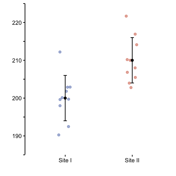
Figure 9.1: Dot plots depicting every data point. The mean height and standard deviation for each site is drawn in black.
Plotting the data is actually the very first thing you need to do when you want to start any sort of analysis! When you afterwards plan to carry out a \(t\)–test, you also need to check the underlying assumption of Normally-distributed data!
Here, we assume that the Martian height at both sites actually is Normally distributed, i.e. \[ X \sim N(\mu_1, \sigma_1) \quad \quad Y \sim N(\mu_2, \sigma_2),\] where \(X\) and \(Y\) denote the random variables ‘Height at site I’ and ‘Height at site II’, respectively.
We are interested in whether the mean Martian height is different between the sites.
Exercise Write down the null hypothesis \(H_0\) and the alternative hypothesis \(H_1\) we wish to test given we want to perform a two–sided test! Hint: use the two (unknown) site mean values \(\mu_1\) and \(\mu_2\).
Now that we know what the null and alternative hypotheses are, let’s think about the signal–to–noise ratio we are interested in here. Remember in the previous chapter we had the (one–sample) situation where our hypotheses had the form \[ H_0: \mu = 195 \quad \quad \mbox{versus} \quad \quad H_1: \mu \neq 195.\] In that situation, we looked at
\[\frac{\mbox{signal}}{\mbox{noise}} = \frac{\mbox{(observed value - hypothesised value)} }{\mbox{scale factor}} = \frac{\bar{X} - \mu_0}{S/\sqrt{n}}\]
which was our \(t\)–statistic that, under the premise of a true \(H_0\), followed a \(t\)–distribution with \(n-1\) degrees of freedom. To test whether the signal was big enough to reject \(H_0\) in our sample, we just needed to plug in our sample estimates \(\bar{x}\) and \(s\), and see where the resulting value \(t = (\bar{x} - \mu_0)/(s/\sqrt{n})\) sits on the \(t_{n-1}\)–distribution.
Here, the situation is slightly more complicated because we have two Normal distributions and four parameters that we somehow must account for. One trick is to rewrite our hypotheses in a way that looks more similar to the one in the one–sample situation: \[ H_0: \mu_1 - \mu_2 = 0 \quad \quad \mbox{versus} \quad \quad H_1: \mu_1 - \mu_2 \neq 0.\]
This formulation emphasises that it is the difference between the means \(\mu_1 - \mu_2\) we are interested in here. With this, it is easy to see that the ingredients for our test statistic are
observed value: We cannot observe the difference between the two population means directly, but like in the one–sample situation we can estimate it using the sample means. Hence we look at \(\bar{x}_1 - \bar{x}_2\) which is an estimate for \(\mu_1 - \mu_2\).
hypothesised value: The hypothesised value is zero (which again corresponds to the state of boredom).
scale factor: In the one–sample situation the scale factor was the \(SEM\), i.e. the standard deviation of the sample mean \(sd(\bar{X})\) which measures the precision that is associated with estimating the population mean by the sample mean. Here, we need the standard deviation of \(\bar{X}_1 - \bar{X}_2\) which is the estimate we are interested in now. Let’s call this \(sd(\bar{X}_1 - \bar{X}_2)\) for now.
From the above, we can now derive the form of the test statistic we are interested in here:
\[\frac{\mbox{signal}}{\mbox{noise}} = \frac{\text{(observed value - hypothesised value)} }{\text{scale factor}} = \frac{(\bar{X}_1 - \bar{X}_2) - 0}{sd(\bar{X}_1 - \bar{X}_2)} = \frac{\bar{X}_1 - \bar{X}_2}{sd(\bar{X}_1 - \bar{X}_2)}.\]
Easy! However, we are not quite out of the woods yet, we still don’t know the form of \(sd(\bar{X}_1 - \bar{X}_2)\) and we also don’t know the null distribution of the test statistic.62
Actually, there are different versions of \(sd(\bar{X}_1 - \bar{X}_2)\) depending on the nature of your data, and these versions also determine which \(t\)–distribution you should use. We’ll go through the three most important versions in this workshop.
9.1 Version 1 – unequal variances test
The most general form of the two–sample \(t\)–test is called Welch’s variant for unequal variances.63 The ‘unequal variances’ refers to the population parameters \(\sigma_1^2\) and \(\sigma_2^2\). You don’t know them of course, but if the corresponding estimates \(s_1^2\) and \(s_2^2\) obtained from the sample are quite different, it’s unlikely that \(\sigma_1^2 = \sigma_2^2\). In this case, \(sd(\bar{X}_1 - \bar{X}_2)\) has the form
\[sd(\bar{X_1} - \bar{X_2}) = \sqrt{{S_1^2 \over n_1} + {S_2^2 \over n_2}}.\]
We won’t get into the reasons for this, but the form of this formula shouldn’t seem too absurd when you remember that in the one–sample situation the scale factor had the form \(SEM = \sqrt{S^2/n}\). With the the above formula plugged in, the entire \(t\)–statistic looks like
\[ t = \frac{\bar{X}_1 - \bar{X}_2}{\sqrt{{S_1^2 \over n_1} + {S_2^2 \over n_2}}} \]
If we plug the values of our Martian height example in the equation, we find the \(t\)–statistic
\[t = \frac{(200-210)} {\sqrt{(\frac{6^2}{10})+(\frac{6^2}{10})}} = \frac{-10}{2.68} = -3.73.\]
Under the null hypothesis \(H_0: \mu_1 - \mu_2 = 0\), it follows a \(t\)–distribution. In the case of assuming unequal variance, the degrees of freedom have quite a complicated form
\[\mathrm{d.f.} = \frac{(s_1^2/n_1 + s_2^2/n_2)^2}{(s_1^2/n_1)^2/(n_1-1) + (s_2^2/n_2)^2/(n_2-1)}.\]
For our example, there are 18 degrees of freedom. Remember, the \(p\)–value is equal to the area under the null distribution for all values that are further from zero, in either direction than the \(t\)–value we observed. This is illustrated in Figure ??. The \(t\)–statistic is really far from 0, so the corresponding \(p\)–value is very low.
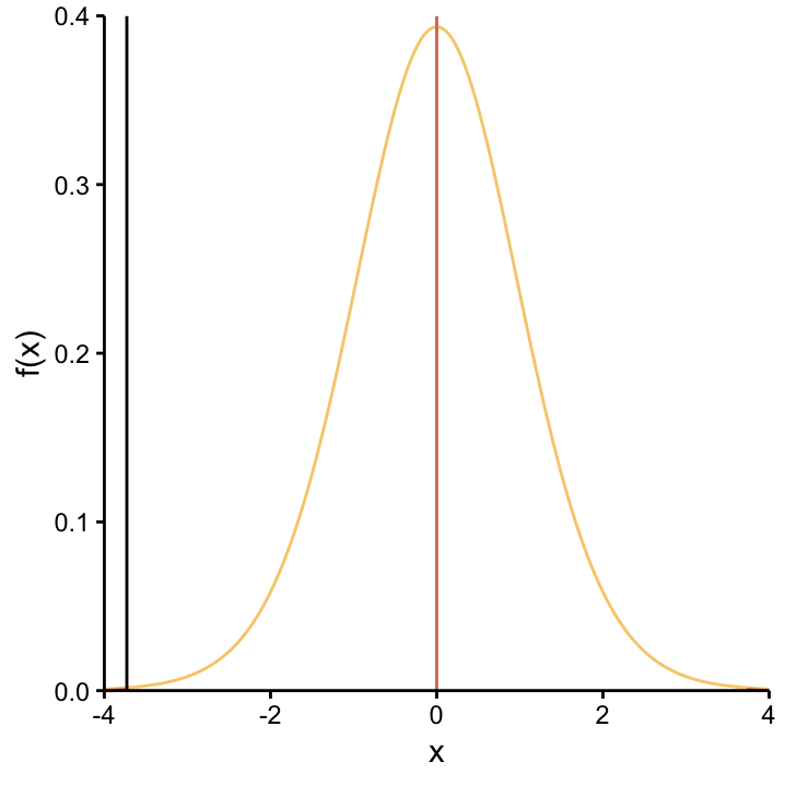 The distribution of the \(t\)–statistic under the null hypothesis \(H_0: \mu_1 - \mu_2 = 0\) is the \(t_{18}\)–distribution. The position of our observed value for this statistic is shown by the red dashed line. To calculate the \(p\)–value, the area under the curve is summed for both tails of the distribution because we decided to use a two–sided test.
In principle this is it – Welch’s variant covered!! However, recall that \(s_1 = s_2 = 6\) cm for our example, so in reality it actually seems not unlikely that \(\sigma_1 = \sigma_2\) in which case we can use a version of the the two–sample \(t\)–test that is build on this assumption. So to show the impact of different standard devations in the two groups, consider two other scenarios, where all the parameters are the same as before except now, \(s_2 = 8\) cm (scenario 2) and \(s_2 = 10\) cm (scenario 2), cf. Table 9.2.
| Parameter | Scenario 1 | Scenario 2 | Scenario 3 |
|---|---|---|---|
| Group 1 (\(\bar{x}, s\)) | (200, 6) | (200, 6) | (200, 6) |
| Group 2 (\(\bar{x}, s\)) | (210, 6) | (210, 8) | (210, 10) |
| t-statistic | -3.73 | -3.16 | -2.71 |
| Degrees of Freedom | 18 | 16.68 | 14.73 |
| \(p\)-value | 0.002 | 0.006 | 0.016 |
These three scenarios are plotted in Figure 9.2, and the results of Welch’s two-sample \(t\)–tests for each scenario are summarised in Table 9.2.
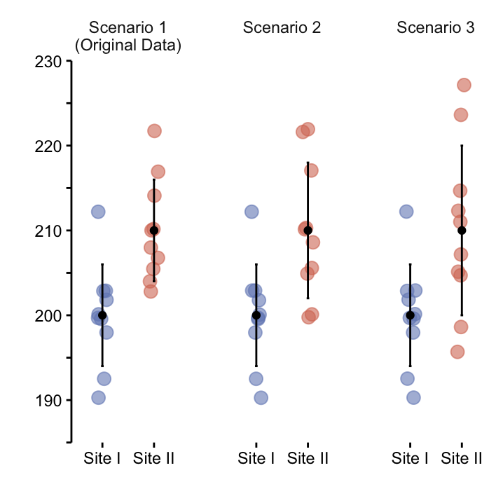
Figure 9.2: Mean with standard deviation.
To consider the effects of increasing \(\sigma_2\), so that \(\sigma_2 \neq \sigma_1\), we compare two simulations with our original scenario, where \(\sigma_2 = \sigma_1\).
What can we deduce from this table? As \(s_2\) increases, keeping all other parameters constant, two things happen. Both the degrees of freedom and the test statistic decrease. Both of these changes have the consequence of increasing the \(p\)-value. This result makes sense, since the large variance in one group precludes a clear distinction between the two groups. A simple way to understand this is that the error bars have a greater overlap, as seen in Figure 9.2.
Notice that we can still get a very small \(p\)–value with overlapping error bars! It is a common misconception that overlapping errors correspond to high, i.e. non-significant \(p\)–values.
Exercise How to you interpret the \(p\)–values above? What’s your conclusion regarding the null hypothesis?
9.2 Version 2 – equal variances
Mr. Welch’s version of the two–sample \(t\)–test didn’t have any restriction regarding the two population variances \(\sigma_1^2\) and \(\sigma_2^2\), and essentially this resulted in a scale factor \(sd(\bar{X}_1 - \bar{X}_2)\), i.e. the noise in the denominator of our signal–to–noise ratio, where each of the two variances were estimated separately. However, if you can assume that the two groups have the some population variance, the situation is a bit different, because in that case your underlying assumption is
\[ X \sim N(\mu_1, \sigma^2) \quad \quad Y \sim N(\mu_2, \sigma^2).\]
So there is only one variance that you need to estimate! And because it’s the same for both groups, you can use a combined form to estimate the common variance as
\[S^2_{pooled} = \frac{(n_1-1)S_{1}^2+(n_2-1)S_{2}^2}{n_1+n_2-2}.\]
With this, the common scale factor has the form
\[sd(\bar{X}_1 - \bar{X}_2) = S_{pooled} \cdot \sqrt{\frac{1}{n_1}+\frac{1}{n_2}}, \]
and the test statistic becomes
\[t = \frac{\bar{X}_1 - \bar{X}_2 }{\sqrt{\frac{(n_1-1)S_{1}^2+(n_2-1)S_{2}^2}{n_1+n_2-2}}\cdot \sqrt{\frac{1}{n_1}+\frac{1}{n_2}}}.\]
Under the null hypothesis it follows a \(t\)–distribution with \(n_1 + n_2 - 2\) degrees of freedom. In our example that would be \(10+10-2=18\). Table 9.3 summarises the results for all three scenarios. We see that the main difference to Table 9.2 is that the degrees of freedom remains constant. Also in each scenario, it is at least as large is the one in Table 9.2 where it decreases as the difference in variance between the groups increases.
| Parameter | Scenario 1 | Scenario 2 | Scenario 3 |
|---|---|---|---|
| Group 1 (\(\bar{x}, s\)) | (200, 6) | (200, 6) | (200, 6) |
| Group 2 (\(\bar{x}, s\)) | (210, 6) | (210, 8) | (210, 10) |
| t-statistic | -3.73 | -3.16 | -2.71 |
| Degrees of Freedom | 18 | 18 | 18 |
| \(p\)-value | 0.002 | 0.005 | 0.014 |
So what’s the effect of assuming a constant variance in both groups? Recall that higher degrees of freedom means that the \(t\)–distribution more closely resembles the standard Normal distribution. This in turn results in lighter tails64. Like in the previous chapter, these lighter tails have to do with the smaller amount of uncertainty that is inherent in the test procedure. Here, the explanation for this is that we need to estimate only one variance parameter when we assume a common variance for both groups. In general, this will result in smaller \(p\)–values for the same signal–to–noise ratio.
This simulation may lead you to conclude that you should always assume equal variance, since that will result in a lower \(p\)-value. However, a word of warning: if the variances are equal, your procedure will be more precise, BUT if they are unequal, you spuriously remove uncertainty, which will result in an inflated type I error rate!
An obvious question is how can you determine if you can assume equal variances. For example, the \(F\)–test is designed for just that.65 However, testing the assumptions with yet another test that also has assumptions is not really optimal. Where do you stop testing assumptions once you are in that loop of testing test assumptions by testing?! The recommendation we give is to eyeball your data to judge whether the assumption of equal variances in your two groups seems OK. If it’s unclear, use the Welch variant of the two–sample t–test as the conservative option.
In this simulation, both the sample sizes and the sample means were held constant in the three scenarios. If these values differ, we begin to see further differences between the two methods. Use the two-sample t-test web app to explore the scenarios presented in this section. Also explore the effect of varying sample sizes.
9.3 Version 3 – paired data
The last type of \(t\)–test to consider is when the data are paired. This means that we measured the same continuous variable twice in the same individual, for example under two different conditions. In our Martian exaple, the continuous variable we will use is the time to run 100 m. We have already measured this value on Mars, so after returning to Earth, we decided to let our Martians run again. Now we’d like to compare the time on Mars to that on Earth. Therefore, our dataset has the form shown in Table 9.4.
| Martian | Mars (s) | Earth (s) |
|---|---|---|
| 1 | 23.25 | 18.98 |
| 2 | 27.44 | 19.19 |
| 3 | 22.12 | 13.39 |
| 4 | 16.34 | 10.93 |
| … | … | … |
| 9 | 21.32 | 18.18 |
| 10 | 20.84 | 16.17 |
Here, we will restrict our analysis to the 10 Martians from site I. As we measures each Martian twice, we are dealing with 20 data-points. Importantly, however, they are not independent. Instead, they come in pairs, and we can assume that these pairs are independent, since they come from different Martians. This data situation is is shown graphically in Figure 9.3. As each measurement on Earth has a corresponding measurement on Mars, it makes sense to connect values within each pair. In a situation like this, you have paired data and should run a paired \(t\)–test where we are primarily interested in the change in the measured value between the two states of the same individual.66
What does that mean? Essentially, we are more interested in the slope of the line than the actual values. Before, we were interested in the yellow and red dots in Figure 9.3, now we are interested in the black lines. Once we understand that we have paired data, we realise that we are actually dealing with a one–sample situation again, because we have a single sample of slopes! This is shown in Figure PairedSeries where the difference between paired values is plotted.
Just like in the one–sample \(t\)–test, the underlying assumption is that the slopes are Normally-distributed, and the null hypothesis is that the mean of the slopes is zero! The test statistic has the same form as that for the one–sample \(t\)–test we saw in chapter ??, and its null distribution again is \(t_{n-1}\). The results of our paired \(t\)–test (or a one-sample \(t\)–test on the slopes, if you like) are summarised in the following table.
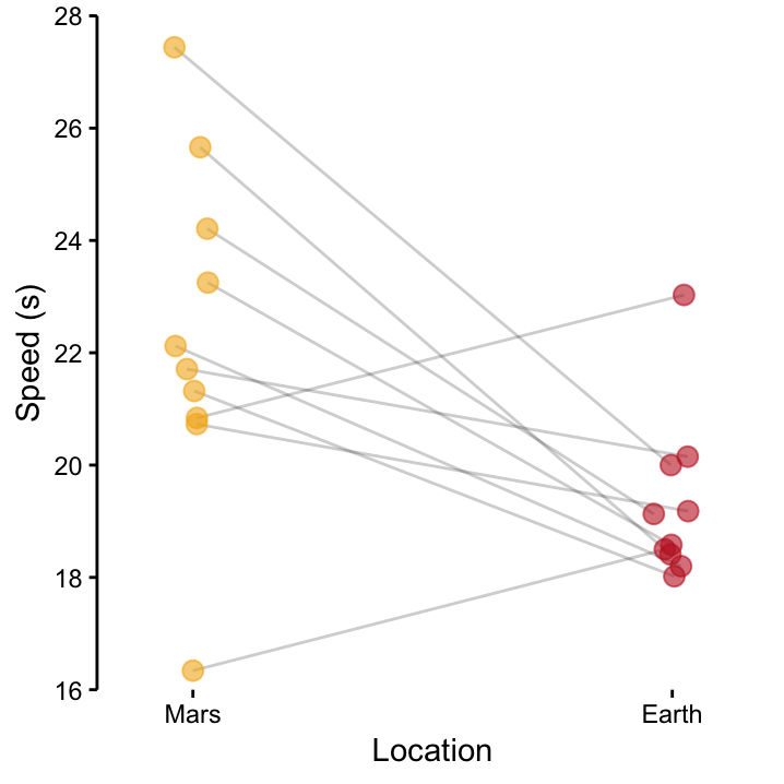
Figure 9.3: Paired data for Martian 100 m trials: The black lines connect the speed on Mars and that on Earth that were measured for each of our 10 Martians from site I.
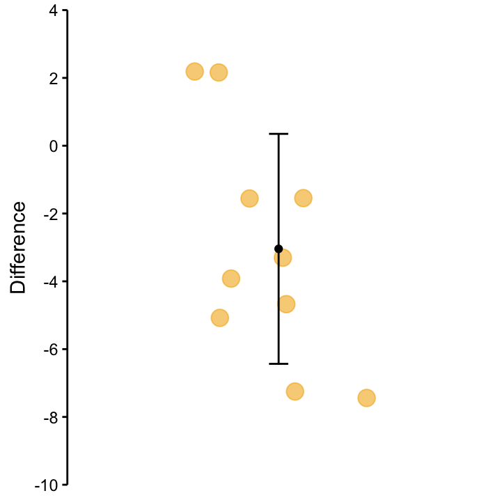
Figure 9.4: Differences between speed on Mars and speed on Earth for the 10 Martians. The values correspond to the slopes on the black lines in the previous figure.
| Test | One Sample t-test |
| Sample mean | -3 |
| Hypothesised value | 0 |
| t-statistic | -2.8 |
| Direction of test | Two-sided |
| Degrees of Freedom | 9 |
| p-value | 0.02 |
| 95% Confidence Interval | (-5.47, -0.62) |
Given we’re still talking about \(t\)–tests, it’s not hard to guess that the null distribution that we’re after will be a \(t\)–distribution. The real question therefore is ‘what’s the correct degrees of freedom’?↩
Good old Mr. Welch wrote the corresponding paper in 1948, not that long ago when you think about it. Stats really is a very young discipline! Welch, B. L. (1947). “The generalization of Student’s problem when several different population variances are involved”. Biometrika 34.↩
The expression ‘light tail’ in the context of a statistical distribution refers to the distributions that have high values around zero and fall off quickly when you move away from zero. For \(t\)–distributions, the tail gets lighter and lighter if you increase the degrees of freedom. Use the \(t\)–distribution app to convince yourself about this.↩
We saw this already when we discussed testing for Normality on page ??.↩
This is actually a much nicer situation because this is more direcly what we were interested in. We don’t have to worry about potential confounding effects, e.g. if by chance the group on Mars contained the Martians that would have been fast on Earth as well!↩