Chapter 11 Linear Regression - Comparing two Continuous Variables
11.1 Part 2 – The F-test Version
So far we have learned how to use a \(t\)–test to find out if looking at an additional variable \(X\) helps us to explain the variation of a variable \(Y\), i.e. if we can improve our predictions of \(Y\) when we know what’s going on with \(X\). If the test is not significant, it means that there is no evidence in the data against the null hypothesis \(H_0: \beta_1 = 0\). This in turn means that we cannot confidently find a line that better explains \(Y\) than the horizontal line showning the mean of y.
Reminding ourselves about this graphical interpretation gives us the opportunity to derive a different method of testing \(H_0: \beta_1 = 0\) which is called \(F\)–test. In the current example, the \(F\)–test is equivalent to the \(t\)–test. Therefore, the following considerations won’t change our conclusions, but they will help us to understand how ANOVA (the topic of the next chapter) is related to linear regression.
If our data offer no evidence against \(H_0\) then we expect that the \(SSR\)73 for the null model (i.e. the horizontal line through \(\bar{y}\)) won’t be much different than the \(SSR\) for our OLS solution (i.e. the line we get by calculating \(\hat \beta_1\) and \(\hat \beta_0\) from the data). As both of these numbers are important, the \(SSR\) for the null model is commonly called \(SST\) (total sum of squares) whereas \(SSR\) specifically denotes the sum of the squared residuals of the OLS solution.
Both numbers are shown in Figure 11.1.
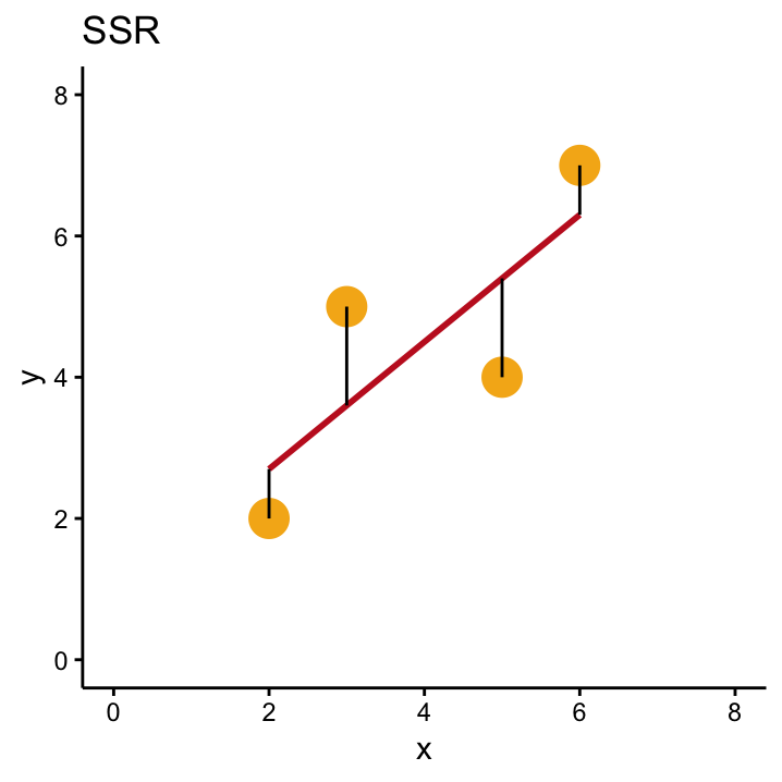
Figure 11.1: A comparison of SSR, SST and SSM in our simple example with four data points.
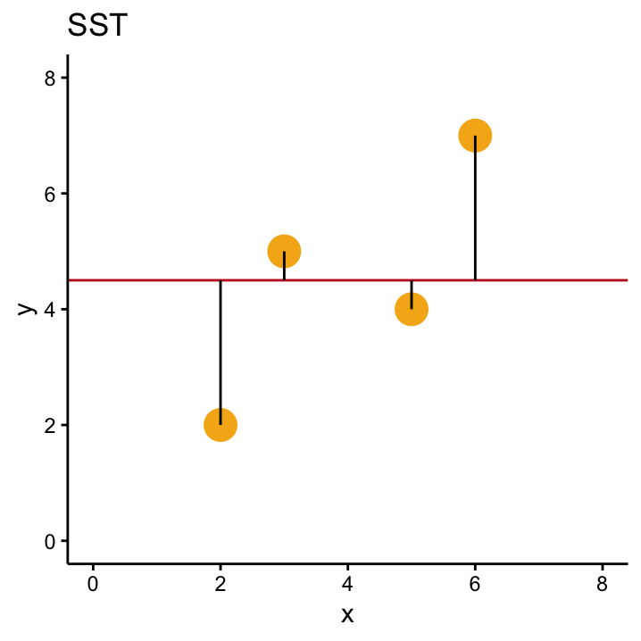
Figure 11.1: A comparison of SSR, SST and SSM in our simple example with four data points.
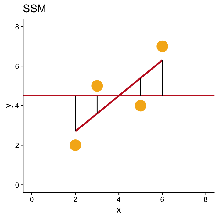
Figure 11.1: A comparison of SSR, SST and SSM in our simple example with four data points.
Independent of the example, we know that the OLS solution will overall have smaller residuals than the the null model, because the OLS line is specifically designed to be the line that minimises this criterion. This means that \(SST\) is always bigger than \(SSR\), no matter what the data look like which in turn means that \(SST - SSR\) will always be greater than zero. This number also has its own name, model sum of squares \(SSM\), and it is depicted in the right–hand–side of Figure 11.1.
The actual values of the three quantities for our example are \(SSM\) = 8.1, \(SST\) = 13, and \(SSR\) = 4.9. In general, \(SST\), \(SSR\) and \(SSM\) play a big role for the \(F\)–test and also in the following chapter, so let’s reiterate what we know about them:
- SST Total sum of squares, i.e. the sum of the squared distances between each point \(y_i\) and the horizontal null model \(\bar{y}\)
\[ SST = \sum_{i=1}^{n}(y_{i}-\bar{y})^{2}.\] It equals the (unscaled)74 variance of the observed \(y\)–values.
- SSR Residual sum of squares, i.e. the sum of the squared distances between each point \(y_i\) and the OLS model \(\hat y_i\)
\[SSR =\sum_{i=1}^{n}(y_{i}-(\hat \beta_0 + \hat \beta_1 x_i))^{2} =\sum_{i=1}^{n}(y_{i}-\hat y_i)^{2}.\]
This number is always smaller than \(SST\). It can be interpreted as the variance that cannot be explained by the OLS line.
- SSM Model sum of squares, i.e. the sum of the squared distances between the OLS model \(\hat y_i\) and the \(H_0\), \(\bar{y}\)
\[SSM =\sum_{i=1}^{n}(\bar y -(\hat \beta_0 + \hat \beta_1 x_i))^{2} =\sum_{i=1}^{n}(\bar y-\hat y_i)^{2}.\]
It can be calculated as \(SSM = SST - SSR\) and can be interpreted as the variance in \(Y\) that can be explained by the OLS model.
From \(SSM = SST - SSR\), it follows that another expression for the \(SST\) defined above is75 \[SST = SSM + SSR.\]
A sensible criterion that measures the improvement the OLS line offers over the null model therefore seems to be the proportion of the total variance that can be explained by the OLS model. This percentage can be calculated as \(SSM/SST\). Hold this thought! We’ll see later that this number is indeed used as a goodness-of-fit criterion. For the \(F\)–test we talk about here, a similar rationale is used: if the OLS line offers a big improvement over the null model, then the variance explained by the OLS model should be much bigger than the variance not explained by it. Therefore \(SSM\) should be bigger than \(SSR\) if we want the reject the null hypothesis \(H_0: \beta_1 = 0\).
This is basically what the \(F\)–test looks at. However, in order to also take into account the sample size, we don’t compare the raw \(SSM\) and \(SSR\), but scaled versions of it which are called mean sums of squares of the model \(MSM\) and mean sums of squares of the residual which are calculated as76
\[ MSM = \frac{SSM}{1} \quad \quad \mbox{AND} \quad \quad MSR = \frac{SSR}{n-2}\] The ratio of these two numbers is called the \(F\)–statistic.
The above table shows all numbers we talked about in the context of our little example. We already said that \(SSM\) = 8.1 and \(SSR\) = 4.9. As the sample size is \(n=4\) in this case, we get \(MSM = 8.1/1 = 8.1\) and \(MSR = 4.9/2 = 2.45\). This gives us an observed \(F\)–statistic of \(F = MSM/MSR = 3.31\). If this value is large, then the variance explained by the OLS model is big compared to the variance that is left after fitting the model (the numerator is big compared to the denominator). So a large \(F\)–value contains evidence against the null hypothesis that the OLS model isn’t appropriate. But again, how large is large enough to reject \(H_0\)?
In this case, the null distribution that we need to compare our observed value of the test statistic to is the so–called \(F\)–distribution. Like the \(t\)–distribution, its shape depends on degrees of freedom that in turn depend on the sample size. The shape of the \(F\)–distribution in fact depends on two degrees of freedom \(df_1\) and \(df_2\) that correspond to the scaling factors we talked about, i.e. \(df_1 = 1\) and \(df_2 = n-2\). This is illustrated in Figure ??. Here \(df_1 = 1\)77 is held constant and \(df_2\) varies according to different values of \(n\). For each distribution the critical value for an \(\alpha\) level of \(0.05\) is also shown.
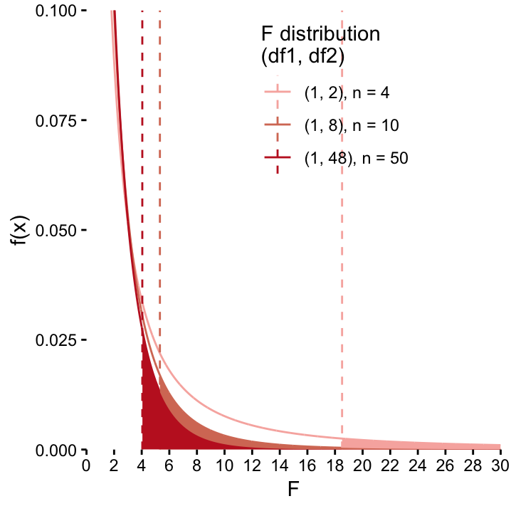 Comparing \(F\)–distributions with variable \(df_2\) parameters. As \(df_2 = n-2\) increases, the curves get flatter which in turn has the effect that critical values for \(\alpha=0.05\) decreases. For small sample size, the observed value of the \(F\)–statistic therefore needs to be really big before we’re convinced that we can reject \(H_0\). For large sample sizes, we have more trust in the data and reject \(H_0\) for smaller observed \(F\)–values. Note that we have already seen this phenomenon when we talked about the \(t\)–distribution.
The \(F\)–distribution that is relevant for our eample is the one where \(df_1 = 1\) and \(df_2 = n-2 = 2\). It is redrawn in Figure ?? together with the observed value \(F=3.31\) (solid line) and the critical value for \(\alpha=0.05\) (dashed line). The red area under the curve shows the \(p\)–value. Just from looking at Figure ?? we know that the \(p\)–value will be greater than 0.05 because our observed \(F\)–value doesn’t exceed the critical value. So as with the \(t\)-test, we cannot reject the null hypothesis for our example. In fact, the \(p\)–values of the \(F\)–test and of the \(t\)–test are exactly the same. This of course is not a coincidence. In the simple case where the effect of one continuous variable \(X\) on one continuous variable \(Y\) is being assessed, the two \(p\)–values are always identical!
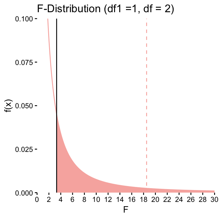 The \(F\)–test (\(df_1 2, df_2 = 2\)) for our hypothetical example. The dashed line represents the critical value, the solid line is the test statistic. The red area under the curve corresponds to the \(p\)–value.
11.2 Summary thus far
In case this was a bit fast for you, don’t worry, the important point here is that in simple linear regression, there are two ways of testing the null hypothesis \(H_0: \beta_1 = 0\):
- calculating \(\hat \beta_1\) together with its standard deviation and perform a \(t\)–test which rejects \(H_0\) if the standard deviation (i.e. the uncertainty) is large compared to the observed value for \(\hat \beta_1\).
- calculating \(SST\), \(SSR\) and \(SSM\) and rejecting \(H_0\) if the (scaled) \(SSM\) is large compared to the (scaled) \(SSR\), i.e. if the linear model we are fitting can explain lots of the variance in \(Y\).
11.3 Goodness-of-fit, correlation and the rest of the world explained
Let’s go back to the start of this chapter, where we said that the line that optimally fits the data at hand is defined as the line that minimises the \(SSR\). Meanwhile we saw that the \(SSR\) we’d get if \(H_0: \beta_1 = 0\) were true is called the \(SST\), and that the improvement that the fitted model (with the slope) has over the null model (with the horizontal line) is called the \(SSM\). In our example we have \(SSM\) = 8.1, \(SST\) = 13, and \(SSR\) = 4.9. Below, you also find a list of the other numbers we encountered during this chapter:
- \(cov(X, Y)\) = 3
- \(s_x\) = 1.83 \(s_y\) = 2.08
- \(s^2_x\) = 3.33 \(s^2_y\) = 4.33
Our goal here is to show that these numbers are all related! And in particular, they all lead to the one thing we haven’t mentioned so far, i.e. the famous correlation coefficient. In our example it takes the value \(r(X, Y)\) = 0.79. Let’s see how we can get there from the numbers above:
- The sample variance of \(Y\) is \[s^2_y = \sum_{i=1^n} (y_i - \bar{y})^2/(n-1) = SST/(n-1)=13/3= 4.33.\]
This is only concerned with the null model, since \(X\) doesn’t occur in the equation
- Once we start also looking at \(X\), we used the covariance, instead of the variance, which is
\[cov(X, Y) = \sum_{i=1}^{n}(x_i-\bar{x})(y_i-\bar{y})/(n-1) = 3. \]
- We saw that the covariance is related to \(\hat \beta_1\), the estimated slope, i.e. it’s just a scaled version of it,
\[\hat \beta_1 = cov(X, Y)/s^2_x = 3/3.33 = 0.9\]
- This is where correlation comes into play. \(\hat \beta_1\) is asymmetrical in the sense that the covariance in the numerator is only standardised by the variance of \(X\) (\(s^2_x\)). Maybe you can appreciate that this standardisation is a bit unfair against \(Y\), since
$s^2_x = s_x s_x $.
If we correct this blatant unfairness by using \(s_y\) as one of the factors in the denominator, we actually get the correlation coefficient!
\[r_{xy} = cov(X, Y)/(s_x \cdot s_y) = 3/(1.83\cdot 2.08) = 0.79.\]
- And to close the circle78, if we square this correlation coefficient, we get the proportion of variance explained by the model, i.e.
\[\begin{eqnarray*} R^2 &=&r^2_{xy} = (cov(X, Y)/(s_x \cdot s_y))^2= (3/(1.83\cdot 2.08))^2 \\ & = & 0.79^2 = 0.62 = 8.1/13 = SSM/SST . \end{eqnarray*}\]
What does this tell us? Actually all three numbers \(cov(X, Y)\), \(r_{xy}\) and \(R^2\) tell us something about the strength of the linear relationship between \(X\) and \(Y\). But they look at it from different angles:
\(cov(X, Y)\) tells us how \(X\) and \(Y\) vary together. If this value is big, a plot of \(X\) against \(Y\) looks like a straight light. If the value is close to zero, it doesn’t , i.e. the strength of the linear relationship is low.
\(r(X, Y)\) essentially measures the same as \(cov(X, Y)\), but in a standardised way because the denominator has the effect that \(r(X, Y)\) can only take values between -1 and 1. The extreme values signify a perfect linear relationship, i.e. the plot \(X\) against \(Y\) is a perfect line. The sign tells us about the direction of the relationship
\(R^2\) is essentially the same, but because the values are squared, information on the direction of the relationship is lost.
And \(\hat \beta_1\)? How does that fit into the picture? The above coefficients are all symmetrical, i.e. it doesn’t matter if you exchange \(X\) and \(Y\). The slope \(\hat \beta_1\) of the optimal line, however, is calculated as \(\hat\beta_1 = \frac{COV(x,y)}{s^2_x}\). Therefore it is inherently asymmetrical as the denominator only looks at the variance in \(X\). As we said, \(\hat \beta_1\) can be defined as the amount of change in \(Y\) when you change \(X\) by one unit. As you can derive from the formula, \(\hat \beta_1\) is big if the covariance of \(X\) and \(Y\)is large compared to the variance in \(X\).
Use the linear regression web app to explore these concepts further!
11.4 Martian examples
Let’s reiterate what we learned with a Martian example. Figure 11.2 shows the relationship between the height of the Martians and the time they need to run 100 meters. The red line displays the OLS solution. The linear regression obviously provides a very good fit, so we expect both the \(t\)–test and the \(F\)–test to give us very small \(p\)–values as the data contain lots of evidence against the null hypothesis that height as nothing to do with speed.
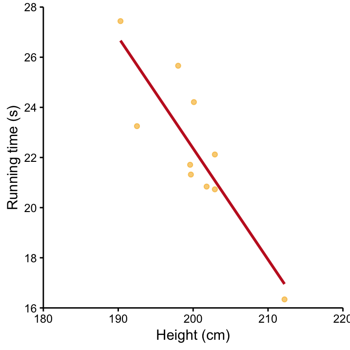
Figure 11.2: Time to run 100m versus Martian height and the associated OLS solution (red line).
Table ?? shows the output of the \(t\)–test. Of particular interest is the second line which contains the test results for the slope. The best guess for the slope is \(\hat \beta_1 = -0.44\), so for each cm increase of the Martians height, we’d predict that they run 0.44 s faster. Given the small amount of scatter around the OLS line, the standard deviation associated with this number is going to be relatively small (indeed it’s 0.09) so that observed value of the \(t\)–statistic is going to be large. Here \(t = -0.44/0.09 = - 5.03\). The corresponding \(p\)–value is \(0.001\) which means that \(t = - 5.03\) is far away from zero that we’re rejecting \(H_0\) at a 5% signifiance level. The evidence in the data against the hypothesis that height doesn’t play a role when it comes to running time is convincing!
The value of \(\hat \beta_0\) is not of interest here, it tells us the predicted speed for a Martian that is 0 cm tall – this is a nice example that you should be careful of how far extrapolation makes sense and which numbers of the output to interpret!
| Estimate | Std. Error | t value | Pr(>|t|) | |
|---|---|---|---|---|
| (Intercept) | 111.0155 | 17.6403 | 6.29 | 0.0002 |
| Height | -0.4433 | 0.0882 | -5.03 | 0.0010 |
The above table gives the same result in terms of the \(F\)–test. As we explored earlier, it gives the same \(p\)–value. The \(F\)–distribution of interest here is shown in Figure ??.
| Df | Sum Sq | Mean Sq | F value | Pr(>F) | |
|---|---|---|---|---|---|
| Height | 1 | 63.56 | 63.56 | 25.28 | 0.0010 |
| Residuals | 8 | 20.12 | 2.51 |
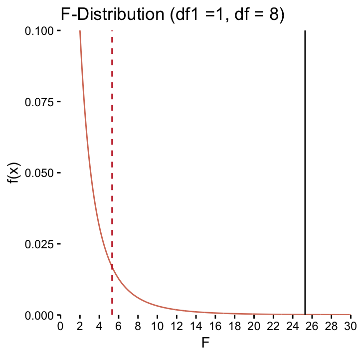 The \(F\)–distribution (\(df_1 2, df_2 = 8\)) for the running time on Mars described by Height. The dashed line represents the critical value, the solid line is the test statistic. The \(p\)–value is very small here, so it’s not visible. It corresponds to the area under the curve to the right of the oberved \(F\)–value.
With this example, the numbers in the table are calculated as \(df_2 = n -2 = 10 - 2 = 8\), \(MSR = SSR/df_2 = 20.12/8 = 2.51\), \(F = MSM/MSR = 63.56/2.51 = 25.28\).
Exercise Can you calculate \(R^2\)?
Now, we’re equipped to understand ANOVA that we’ll cover in the next chapter. You’ll see it’s just a small step from here. Yet another variation on the same theme!!
Recall that the \(SSR\) is the sum of the squared residuals, a measurement of how well our model fits the data.↩
Here, unscaled means that we didn’t divide the variance by \(n-1\), we’ll see why later on in the text.↩
To summarise:\\(SST > SSR\), and,\\(SSM = SST - SSR\), which means that\\(SST = SSM + SSR\)\i.e. The total sum of squares, \(SST\), corresponds to the variability in \(Y\) which is explained by the model (\(SSM\)) plus that which is not explained by the model (\(SSR\)).↩
Scaling is nothing new, recall that for \(s^{2}\), we scaled the sum of squared residuals by \(n-1\). In fact \(s^2\) would be the scaled version of \(SST\). Just like \(SST\) can be divided into \(SSM\) and \(SSR\) we need to divide \(n-1\) into 1 and \(n-2\).↩
For linear regression with two continuous variables we always have \(df_1 = 1\) because we are estimating the same number of \(\beta\) coefficents each time, namely intercept and slope. When we cover ANOVA in the next chapter you’ll see that the general form for the degrees of freedom is \(df_1 = k-1\) and \(df_2 = n-k\), where \(k\) corresponds to the number of coefficients that needs to be estimated in the analysis.↩
The nice relationship \(R^2=r^2_{xy}\) only holds when we are dealing with a single independent variable. \(R^2 = SSM/SST\), however, is a general statement that also holds in multiple linear regression where we have several independent variables.↩