Chapter 7 Estimation in practice - Confidence Intervals

Now that we understand the implications of using \(\bar{X}\) as an estimator, let’s explore what this means in practice.

7.1 The standard error of the mean

The standard error of the mean (\(SEM\)) is widely used and very important as it tells us how precisely we can estimate \(\mu\) using \(\bar{X}\). We want the \(SEM\) to be small, since this means greater precision.

The good new is that we’ve covered the \(SEM\) already in passing, so let’s briefly summarise what we learned so far: The sample mean \(\bar{X}\) has a distribution with mean \(\mu_{\bar{X}} = \mu\) and variance \(\sigma^2_{\bar{X}} = \sigma^2/n\).

From this we immediately arrive at the fact that the standard deviation of the estimator \(\bar X\) can be written as \[ \sigma_{\bar{X}} = \sqrt{\sigma^2_{\bar{X}}} = \sqrt{\sigma^2 /n} = \sigma / \sqrt{n} \] which is the \(SEM\)! That’s all there is to it!

Recall that \(\sigma^2\) denotes the variance of the population, so \(\sigma\) is the population standard deviation. Just like \(\mu\), it usually is unknown so we need to replace it with sample standard deviation \(s\) which we discussed on page var-sq. So the \(SEM\) that you are dealing with in practice is \(SEM = s/ \sqrt{n}\).

Many scientists confuse the standard devation of the sample \(s\) (which is a descriptive statistic) with the \(SEM\) (which is an inferential statistic). This is an important distinction - don’t mix them up!

7.2 The Central Limit Theorem

The term Central limit theorem may sound scary but the underlying concept is very cool and very very useful!³⁴ It states that not only do we know the mean and variance of the estimator \(\bar X\), we actually know its entire distribution!

Recall from the videos in Figures 3010PopSam and 3010PopSamLarge that \(\bar{X}\) has a pleasant-looking symmetrical distribution. As you may have guessed, the central limit theorem (CLT) links the distribution of the sample mean to the Normal distribution. This is very good news, because we spent a lot of time learning stuff about the Normal distribution, and now we can apply everything to the problem of estimating \(\mu\) by \(\bar X\)!

As a formula the CLT looks like this: \[ \bar{X} \stackrel{n \rightarrow \infty}{\sim} N(\mu, \sigma^2/n).\] When we say it in words it simply means “if the sample size \(n\) approaches infinity, the sample mean \(\bar{X}\) is Normally distributed with mean \(\mu\) and variance \(\sigma^2/n\)”. Actually the only scary part that we don’t understand right now is the meaning of “as \(n\) approaches infinity”. If we substitute this part with “if your sample size is big enough” the whole thing is not scary anymore at all. It basically says:

For large sample sizes, the sample mean is Normally distributed.

AMAZING!! The only question that remains is, “how large is large enough?” Many text books answer this question with \(n=30\), but 30 is not a God-given magic number. The truth is that “large enough” depends on the distribution of the variable of interest. To explain this, let’s explore the CLT in our web app.

Use the Central Limit Theorem web app to explore what factors influence the distribution of \(\bar X\). According to the CLT, what are the benefits of having a large sample.

The app shows us that large samples not only ensure that the precision of your estimates increases (by decreasing the variance, and thus the \(SEM\)), but also that \(\bar{X}\) follows a Normal distribution which is very easy to deal with since we know everything about it. This is the power of the CLT!

The Central Limit Theorem states that, if the sample size is large enough, \(\bar{X}\) will be Normally distributed regardless of the underlying distribution of your variable \(X\) (!!!)

7.3 Confidence intervals

The CLT is so important because it provides the basis for many results in inferential statistics. Actually most of what we’ll cover from this point on will have the CLT acting in the background. To start with, the CLT is behind the well–known formula for confidence intervals. To see this, let’s return to our Martians.

For Martian height at site I, we saw that \(\bar{x} = 200\) cm. What can we say about \(\mu\)? We now know that our \(\bar{x}\) depends on the specific sample we’ve taken so it’s very unlikely that the \(\bar{x}\) of our sample of 10 Martians exactly matches the population \(\mu\). Therefore we can’t just report \(\bar{x}\) on its own. We should report a range around \(\bar{x}\) that somehow reflects this uncertainty. This is the purpose of a confidence interval (CI).

Suppose³⁵ we have a large sample, and thus the CLT applies. That means that the distribution of all possible sample means, \(\bar{X}\), can be described by

\[ \bar{X} {\sim} N(\mu, \sigma^2/n).\]

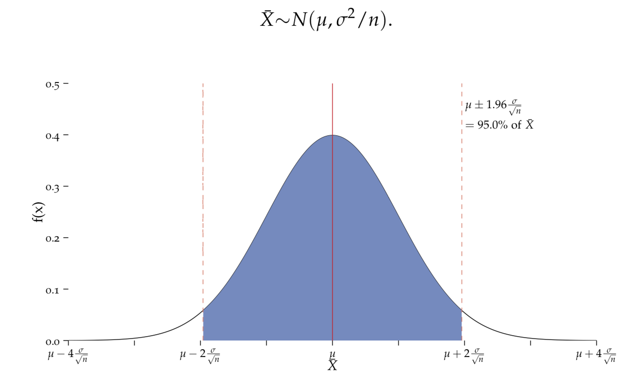
Figure 7.1: Distributions

According to the CLT, the distribution of \(\bar{X}\) is the Normal distribution with a mean \(\mu\) and variance \(\sigma^2/n\). The standard error, \(SEM\), is \(\sigma/\sqrt{n}\), which means that 95% of all possible sample means will fall within the interval \(\mu\pm1.96\frac{\sigma}{\sqrt{n}}\).

Now comes the cool stuff: since \(\bar X\) follows a Normal distribution, we can apply the results from Table Normal_perc. For example we know that 68% of all values fall within the interval \([\mu - \sigma/\sqrt{n} \; , \; \mu + \sigma/\sqrt{n}]\), i.e. 68% of all the samples we can draw from the population will have a mean value \(\bar{x}\) that falls in this interval.³⁶ Similarly,

if the sample size is large enough, there is a 95% chance that the sample mean \(\bar{x}\) lies within \([\mu - 1.96 \cdot \sigma/\sqrt{n} \; , \; \mu + 1.96 \cdot \sigma/\sqrt{n}] = \mu \pm 1.96 \cdot SEM\) (Figure DistSEM).

Let’s imagine that we took 20 independent samples from a population, as shown in Figure DistwithSamples. There will probably be only one of them (5%) that results in a sample mean that falls outside the interval \(\mu \pm 1.96 \cdot SEM\). 95% of all potential sample means will fall in that interval. All of this follows from the CLT.

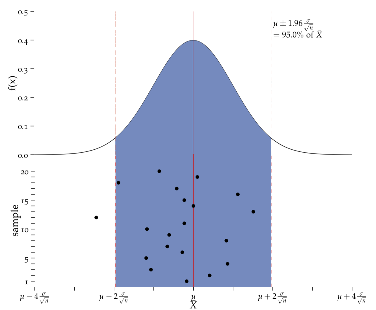
Figure 7.2: Sampling

Top: The distribution of all sample means, \(\bar{X}\), as shown in Figure DistSEM. Bottom: 95% (here 19/20) Of all sample means \(\bar{x}\) are expected to fall within, and 5% (1/20) are expected to not fall within, the interval \(\mu\pm1.96\frac{\sigma}{\sqrt{n}}\).

As you might have realised the interval \(\mu \pm 1.96 \cdot SEM\) looks a bit like the well–known formula for CI 95% – except it’s centered around \(\mu\). Obviuosly this is rather unpractical as \(\mu\) is the unknown quantity that we are trying to estimate. What we have in front of us from the sample is \(\bar x\)!

The trick here is to realise that whenever \(\bar x\) is close enough to \(\mu\) to fall into \(\mu \pm 1.96 \cdot SEM\), the interval \(\bar x \pm 1.96 \cdot SEM\) that is centered around \(\bar x\) will cover \(\mu\). We know that there is a 95% chance for the former to happen so this 95% chance also holds for the latter. 95% of all intervals \(\bar x \pm 1.96 \cdot SEM\) will cover \(\mu\)! This is what we call the 95% confidence interval:

\[\begin{eqnarray}\label{eq:95CI} 95\% CI = \bar{x} \pm 1.96 \cdot SEM. \end{eqnarray}\]

If the sample size is large enough, there is a 95% chance that the interval \(\bar{x} \pm 1.96 \cdot SEM\) covers the true population mean \(\mu\). The width of the interval decreases with larger sample sizes.

³⁷

While this all sounds great, it is important to remember that

We never know which \(\bar{x}\) we have, cf. Figure BlueRedFig. We may have the bad luck to get one of the 5% of \(\bar{x}\) values that fall outside the region \(\mu \pm 1.96 \cdot SEM\) in which case our 95% CI, \(\bar{x} \pm 1.96 \cdot SEM\) will miss \(\mu\).

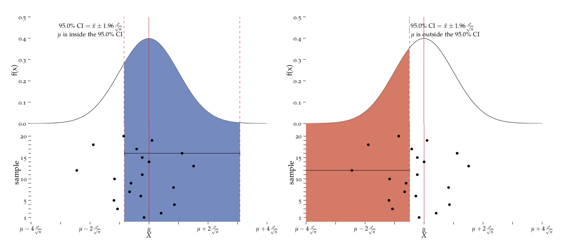
Figure 7.3: Successful and Unsuccessully covering the population mean.

Left: When centering the 95% CI over an \(\bar{x}\), we will cover \(\mu\) 95% of the time. Right: In 5% of the cases, we will fail to cover \(\mu\).

From equation (eq:95CI) we see that the smaller the \(SEM\) is, the narrower is the CI. Conceptually, this should make sense, since you’ve seen that the \(SEM\) reflects the uncertainty that is associated with using \(\bar{X}\) as an estimator for the unknown \(\mu\).

Exercise What can you do to decrease the width of your confidence interval? Hint: think about the \(SEM\)!

Aside from the two parameters that influence the size of \(SEM\) (and thus the CI), there is another factor to consider - the desired level of confidence. So far we have only talked about the 95% CI, but you may also want to be 99% certain that the interval you state covers the true population mean.

Exercise If we increased the CI from 95% to 99%, would the interval get smaller or larger?

Exercise Look at the properties of the normal curve in Table on page DifferentNormalCurves. What CI do scientists refer to when the report \(\bar{x} \pm SEM\) in publications? Hint: Give the percent.

This is pretty much all you need to know about confidence intervals, but there are two points to keep in mind.

We ignored that fact that in any practical situation we don’t know what the population variance \(\sigma^2\) is. That means we also don’t really know the \(SEM\)! However, since we are talking about situations where the sample size is large (otherwise the CLT would not apply), we can quite safely replace \(\sigma^2\) by the sample estimate \(s^2\). We’ll discuss the case when we need to account for the uncertaintly in using \(s^2\) on page sec:the_t_distributiuon.
We deliberately repeated “if your sample size is large enough” many times because all of this holds true only in that case. If your sample size is small, it’s still possible to remedy the situation and come up with similar statements if your variable of interest (or a transformed version) can safely be assumed to be Normally distributed in the population. If you have a small sample size and are not sure if the variable that you are looking at follows a Normal distribution in the population, you know so little about your system that you should be content with sample description or use non–parametric methods some of which we’ll cover later on.

7.4 Sample size calculation for beginners

The previous section tells us that we can be 95% certain that the true mean height of all Martians is covered by the interval \([196.28, 203.72]\). Are you happy with this result? In some cases, the calculated CIs are really unsatisfactorily large, so what can we do to add precision and obtain small confidence intervals? The bad news is that once the study is done, all we can do is accept what we have and aim for more precision next time we do a study. There is, however, a way to influence the width of the confidence interval when you start thinking about it BEFORE you even start conducting the study.

As we have seen, the width of the CI depends on the \(SEM\) which in turn depends on the sample size. Large samples give small \(SEM\)s which give small CIs and therefore high precision. If you know that in your particular case, it’s absolutely important to measure some quantity with a precision that results in a 95% CI of a certain width \(w\), you can just look at formula (eq:95CI) again to see that

\[\begin{eqnarray*} w & = & 2 \times 1.96 \times SEM \\ & = & 3.92 \times SEM \\ & = & 3.92 \times \frac{\sigma}{\sqrt{n}} \end{eqnarray*}\] which means that achieving a width of \(w\) would need a sample size of \[\begin{eqnarray*} \sqrt{n} & = & \frac{3.92 \times \sigma}{w} \\ n & = & \frac{15.37 \times \sigma^2}{w^2} \end{eqnarray*}\]

would do the trick! As expected, this formula tells us that we need large samples if the desired width \(w\) is small (something small in the denominator makes the fraction large) and/or if the variance is large.³⁸

Exercise How can you calculate the sample size required for a 99% CI to have a certain width \(w\)?

7.5 Using error bars in figures

To reiterate some of the things we’ve learned so far about uncertainty and precision, let us consider error bars which put things into a practical context. We are now equipped to critically examine the use of error bars, but before we do so, let’s remind ourselves how they are defined:

Error bars are a graphical representation of the variability of data and are used on graphs to indicate the error, or uncertainty in a reported measurement. They give a general idea of how accurate a measurement is, or conversely, how far from the reported value the true (error free) value might be. Error bars often represent one standard deviation of uncertainty, one standard error, or a certain confidence interval (e.g., a 95% interval).³⁹

Exercise Often you see plots with error bars around the sample mean of the data. What is the true (error free) value in this case?

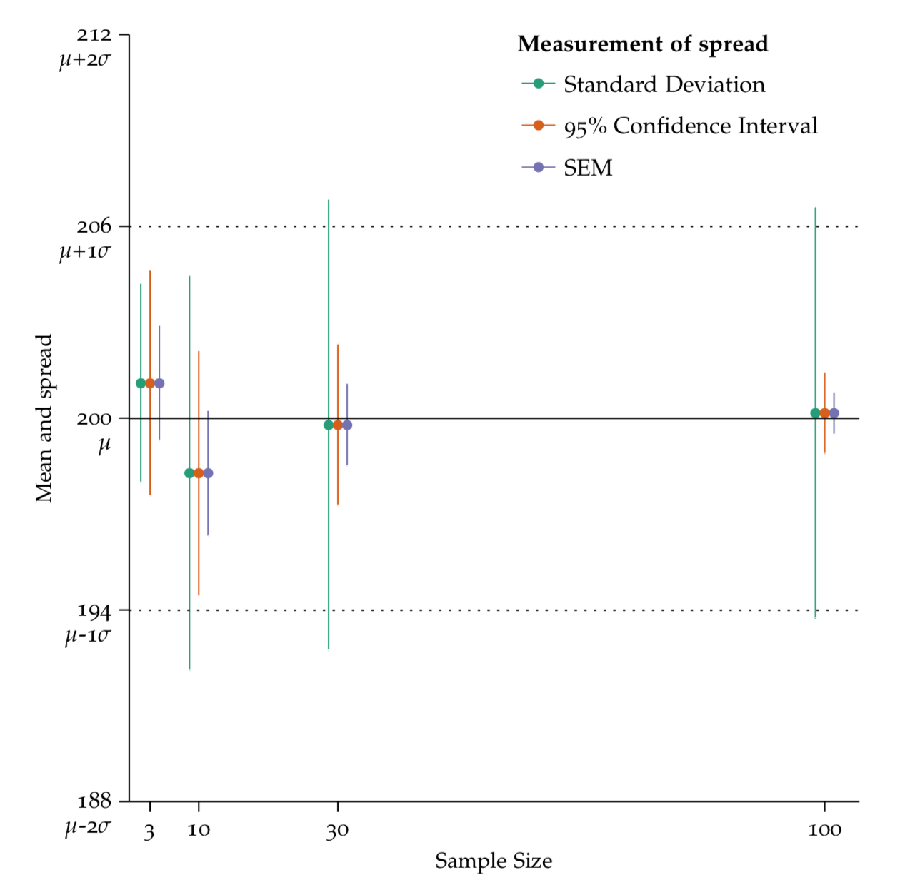
Figure 7.4: Comparing different types of error bars.

The horizontal lines depict our population mean (solid) and standard deviation (dashed) from a simulated population. Selecting samples of different sizes, i.e. 10, 30 or 60 observations, affects error bars in different ways. Standard deviation is relatively stable across sample sizes, whereas the 95% confidence interval and the SEM get smaller as sample size increases.

Geoff Cumming and colleagues have a couple of very informative papers on the topic of error bars.⁴⁰ The authors distinguish between descriptive and inferential error bars.

Exercise Refer to Figure dif-types-spread and fill in Table 7.1. In the type column, indicate if the error bar is descriptive or inferential. In the description column, define, using simple language, what each error bar tells us (no equations or text book definitions!).

Table 7.1: Types of Error bars.
Error Bar	Type	Explanation
Standard Deviation
Standard Error of the mean
95% Confidence Interval

Exercise What should you think if you see a paper that contains a figure with error bars, without specifying what they represent?

To end our discussion about error bars, consider this quote from the GraphPad Prism website⁴¹:

If your goal is to emphasise small and unimportant differences in your data, show your error bars as \(SEM\), and hope that your readers think they are SD. If our goal is to cover-up large differences, show the error bars as the SD for the groups, and hope that your readers think they are \(SEM\)s.

Some word of advice: if you don’t understand the joke, review the differences between SD and SEM.

7.6 95% Confidence Intervals Exercise

Follow this link to enter you values for the in-class exercise.

Depending on who you read, the CLT is the best thing to ever happen to Statistics. It’s like what PCR is to molecular biology, or mayonnaise to french fries. Life just isn’t the same after you discover these things.↩
When we say that the CLT applies, it means that our sample is large enough that we can assume a Normal distribution of the sample means. In this case an \(n\) of 10 is pretty small, but we’ve seen that Normal assumption for the variable height seems justified, so the sample mean will also be Normally distributed.↩
This is exactly what we saw in Figure DifferentNormalCurves and Table Normalperc on page DifferentNormalCurves. The only difference is that the standard deviation that is associated with the mean is \(\sigma/n\) rather then just \(\sigma\).↩
It’s like we’re going on a fishing trip, we cast a net to try and catch \(\mu\). Lucky for us it’s not moving! With a 95% CI, we can catch it 95% of the time, but that means that there’s still a 5% chance we’re going to miss the true \(\mu\)!↩
Caution: in order to use the formula, you need to have an idea of the magnitude of the variance BEFORE you do the study! You could use values from previous similar studies or make some other informed guess.↩
Wikipedia, The Free Encyclopedia, s.v. “Error bar,” (accessed Januar 04, 2018), https://en.wikipedia.org/wiki/Error\_bar.↩
“Error bars in experimental biology”. Geoff Cumming, Fiona Fidler, and David L. Vaux. The Journal of Cell Biology, Vol. 177, No. 1, April 9, 2007, pp 7-11.↩
graphpad.com/guides/prism/6/ statistics/index.htm?statwh entoplotsdvssem.htm↩