Chapter 8 Introduction to Hypothesis Testing

We’ve already come pretty far in our understanding of statistics and have even taken our first steps into the territory of inferential statistics.

8.1 From confidence intervals to hypothesis testing

Confidence intervals and hypothesis testing are close relatives. To see this, let us first remind ourselves how we calculate and interpret confidence intervals. If you have a hard time with the following exercises, refer back to page sec:conf-int.

Exercise Imagine that a 95% confidence interval for the height of Martians at Site I is $[196.28, 203.72]$. Write a sentence that correctly describes this finding.

Exercise What is the observed mean? What is the $SEM$?

To see the connection between confidence intervals and hypothesis testing, image that, before we began our exploration to Mars, we did some background research. It seems that Earthlings have always had a notion of what Martians are supposed to look like (think of Marvin the Martian, pictured). Based on this, we formulate the a priori hypothesis (i.e. an hypothesis that is based on a notion we obtained before we collected the sample) that Martians should on average be $195$ cm tall.

Exercise Based on our sample, do you believe this? Do our data support this hypothesis? Give reasons as to why or why not.

Congratulations! You have just performed a hypothesis test without even noticing! Let’s explain: Recall how we derived the interpretation of the confidence interval above?⁴² Our starting point was the CLT, from which we know that 95% of all sample means $\bar{x}$ that we could have gotten from the population will fall into the interval $\mu \pm 1.96 \cdot SEM$. Then we noted that this implies that 95% of all the intervals $\bar{x} \pm 1.96 \cdot SEM$ will in turn contain the true underlying $\mu$, i.e. for the single confidence interval that you get from your sample, the chance that it covers $\mu$ is 95%.

To highlight the relationship between confidence intervals and hypothesis testing, we can use the exact same trick with one further gimmick which relates to the main difference between the two methods, i.e. the presence of an explicit hypothesis! In our example, the hypothesis is that the true mean Martian height is $195$ cm. An hypothesis of this kind is commonly called null hypothesis. We can write $H_0: \mu=195 cm$.

Now suppose that $H_0$ indeed describes the true state of the world and the mean height of the entire Martian population at Site I really is 195cm. In this case we know from the CLT, that the distribution of the sample mean $\bar{X}$ is⁴³

\[\bar{X} \sim N(195, SEM^2) \quad \mbox{or} \quad \bar{X} \sim N(195, 1.9^2).\]

This implies that 95% of all sample means, $\bar{x}$, would lie in the interval $195 \pm 1.96 \cdot 1.9 = 195 \pm 3.72 = (191.28, 198.72)$, i.e. the chance of observing an $\bar{x}$ outside this interval is only 5%. Therefore, if we do observe an $\bar{x}$ outside of this interval, we are inclined to _reject the null hypothesis- with 95% confidence.

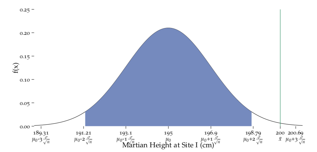
Figure 8.1: Distribution of the sample mean under the null hypothesis.

i.e. under the premise that the mean height in the population is $\mu_0 = 195$. The observed mean value $\bar{x} = 200$, lies outside the region $\mu_0 \pm 1.96 \cdot SEM$ which provides evidence against $H_0$.

This situation is depicted in Figure fig:Draw-normal-testing1 where the green bar shows our observed sample mean $\bar{x} = 200$ and the blue region is the interval $\mu_0 \pm 1.96 \cdot SEM$ that we calculated with our hypothesised value $\mu_0 = 195$ and our $SEM = 1.9$. We see that the probability of observing data like ours (i.e. data that yield an observed sample mean $\bar{x} = 200$) under the premise of $H_0$ is not very big. In fact, it’s smaller than 5% as $\bar{x}$ lies outside the blue region. Therefore the data provide evidence against this null hypothesis. We would reject it with 95% confidence!

Exercise Would you reject $H_0: \mu = 196 cm$?

The cool thing is that the above reasoning holds for all hypothesised values $\mu_0$ that are outside of the 95% confidence interval. This is because if $\mu_0$ does not lie inside $\bar{x} \pm 1.96 \cdot SEM$, it’s also⁴⁴ true that $\bar{x}$ does not lie inside $\mu_0 \pm 1.96 \cdot SEM$! So in our example, even without being much of a mathematician, you can say right away that all hypothesised mean values outside the 95% CI range $[196.28, 203.72]$ are not consistent with our data. All values within the confidence interval, however, remain potential candidates for the true mean Martian height in our population (at site I). Magic!

Before we move on deeper into the realm of hypothesis testing, let’s summarise what we’ve learned so far about the relationship between confidence intervals and hypothesis testing:

A confidence interval contains a range of possible values for the parameter of interest that are consistent with the data, i.e. that are credible possibilities for the true underlying population value of the parameter.
In significance tests only one possible value for the parameter, called the hypothesised value, is tested. We determine whether our data are consistent with the proposition that the hypothesised value is the true underlying parameter value.
All values outside the⁴⁵ confidence interval would be rejected if they were hypothesised in a significance test. The confidence level determines the certainty with which you’d reject the null hypothesis, e.g. all values outside a 95% confidence interval can be rejected if we accept that there is a 5% chance that we make a mistake.

8.2 A general recipe for hypothesis testing

Understanding the previous paragraph is crucial, as it provides a general recipe for hypothesis tesing that ermerges when we disassemble the steps that we took to reach a decision about our null hypothesis:

Pretend that your null hypothesis is true: in our example we pretended that $\mu_0=195$ cm is the true underlying mean height in the Martian population at site I.
Derive the distribution of your statistic under $H_0$: if $\mu_0=195$ cm is true, we know that $\bar{X} \sim N(195, SEM^2)$, i.e. $\bar{X} \sim N(195, 1.9^2)$.
Assess how unlikely it is that you would see your data under the premise of $H_0$: in our example, the probability to obtain a sample with a mean height of $\bar{x} = 200$ cm is less than 5%.
Reach a decision: as we considered ‘less then 5%’ above to be small enough, we concluded that there is enough evidence in the data to reject $H_0$.

In principle, this is it – chapter closed! We’ll spend a bit more time on this topic though to investigate a few subtleties and introduce some official stats jargon.

8.3 The signal and the noise – what we do in hypothesis testing

At the beginning of our chapter on estimation on page chap:estimation, we stated that in hypothesis testing, we address the general question ‘In case I see something interesting in my data, is the effect real (i.e. due to some systematic pattern) or is it just due to chance?’. Let’s see what we meant by this!

Exercise In our example where we observe a mean height of $\bar{x} = 200$ cm, and we want to assess the credibility of the null hypothesis $H_0: \mu = 195$ cm, what do you think is the effect that we talk about?

Here, the effect is the fact that the sample mean isn’t equal to the hypothesised population mean, i.e. $\bar{x} - \mu_0 \neq 0$. In hypothesis testing we want to know if this effect is real (i.e. if our data and the null hypothesis are far enough apart to count as a systematic pattern) or if the distance $\bar{x} - \mu_0$ we observe could have occurred just by chance despite $\mu_0$ being the true underlying value.

If you rephrase this question a bit, you are asking whether there is a real signal among the noise we have in the data, where the signal corresponds to the effect we defined above and the noise corresponds to the random sampling variation.

In our example, the reason why observing $\bar{x} = 200$ cm is so unlikely under $H_0: \mu = 195$ cm is that the difference between the two values (i.e. the signal $\bar{x} - \mu_0$) is quite a bit higher than the $SEM$ which, as we know, can also be seen as the noise we have in estimating $\mu$ using the sample mean, $\bar{x}$. The signal to noise ratio we are looking at here can therefore be written as

\[ \frac{\mbox{signal}}{\mbox{noise}} = \frac{\bar{x} - \mu_0}{SEM} = \frac{200 - 195}{1.9} = 2.64. \]

Does that remind you of something? It should! This is essentially what you saw when we described $Z$–scores!⁴⁶ This is really good news because it provides us with a standardised way to assess whether the signal to noise ratio is big enough to reject the null hypothesis! Instead of writing $\bar{X} \sim N(195, 1.9^2)$ under the null hypothesis (cf. point 2 in section sec:recipeTesting), we can equivalently state that \[ \frac{\bar{X} - \mu_0}{SEM} \, \stackrel{H_0}{\sim} \, N(0,1). \] This means that if we want to know if our observed signal–to–noise ratio, $(200 - 195)/1.9 = 2.64$ is big, i.e. unlikely to have occurred under $H_0$, we can just have a look where it sits on the standard normal curve! If it’s far off from zero, we are inclined to reject $H_0$ and if it’s close to the center, the hypothesised value $\mu_0 = 195$ is a plausible value for the true mean height!

This is a neat standardised way to carry out step 3 in section sec:recipeTesting! It is depicted in Figure fig:Draw-normal-testing2 where our observed $z-$score⁴⁷ of 2.64 lies outside the interval [-1.96, 1.96] which, as you may recall, is the interval where 95% of all values fall when the underlying distribution if the standard normal distribution. As before, this means if $\mu_0 = 195$ really was the true population mean, it would be less than 5% likely to observe $\bar{x}=200$. However, instead of wondering if $\bar{x} = 200$ and $\mu_0 = 195$ are far apart given the sampling variation, we can right away say that $z=2.64$ is far off on the standard normal curve!⁴⁸

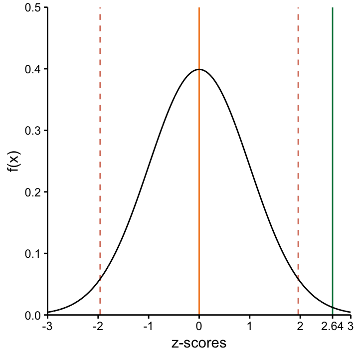
fig:Draw-normal-testing2 Distribution of the signal–to–noise ratio under the null hypothesis. The observed signal–to–noise ratio $z= 2.64$ lies outside the region [-1.96, 1.96] which provides evidence that the signal is bigger than expected by chance and the null hypothesis should be rejected.

8.4 The test statistic and the null distribution

In the previous paragraph we have, in passing, introduced very important concepts that deserve their own section, namely the test statistic and the null distribution. Both are crucial ingredients in hypothesis testing so let’s mention them explicitly!

In our example, the test statistic was $(\bar{X} - \mu_0)/SEM$. Under the null hypothesis, we know that it follows a standard normal distribution which is the null distribution in this case. In more general terms we can write:

The test statistic of a hypothesis test measures the discrepancy between what you observe and what you expect to see under the null hypothesis. It has this general form⁴⁹

\[\frac{\mbox{(observed value)} - H_0}{\mbox{Scale factor}} \quad = \quad \frac{\mbox{signal}}{\mbox{noise}}.\]

Under $H_0$ it follows a distribution (called the null distribution) that assigns a lot of probability to the region around zero, because if $H_0$ is true, what you observe shouldn’t be all that different from zero. Therefore we can conclude that:

The further away from zero the observed value of the test statistic is, the more evidence the data provide against $H_0$!

This last statement is closely related to the definition of a $p$–value, but before we go there, we have one confession to make.

8.5 The problem of not knowing $\sigma$ – the t-distribution

Do you recall the definition of the $SEM$? It’s the standard deviation of the population $\sigma$ divided by the square root of your sample size $n$. If you plug this into the generic formula for the test statistic above, we get $(\bar{X} - \mu_0)/SEM = (\bar{X} - \mu_0)/(\sigma/\sqrt{n})$. The problem is, however, that we never know $\sigma$. So far, we have conveniently ignored this fact, but now it’s time to face reality. How can we deal with this?

One obvious solution is to estimate it from the sample! There is some good news and some bad news about this approach. Good news first: if we replace $\sigma$ by its estimator $S$ we get \[\frac{\bar{X} - \mu_0}{S/\sqrt{n}} \stackrel{H_0}{\sim} t_{n-1},\] i.e. a test statistic that looks very similar to the one we talked about, but apparently it follows a different distribution. This distribution is the famous $t$–distribution! Actually, it is very similar to the standard Normal distribution. However, there are two key differences to note. The t-distribution is:

Flatter and has than the standard normal distribution.
Influenced by a parameter that is called , which in this case is $n-1$.

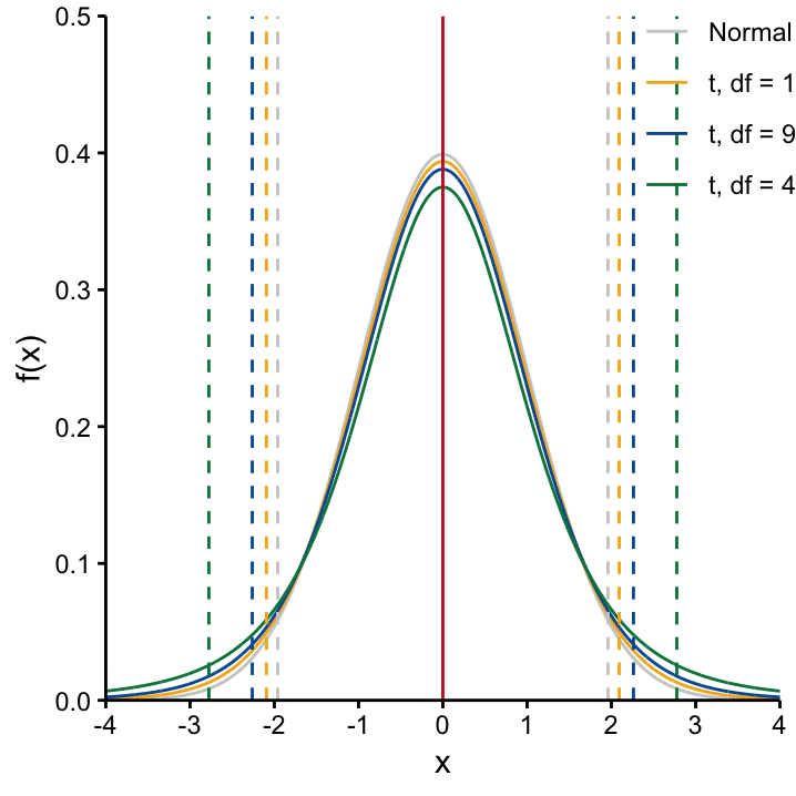
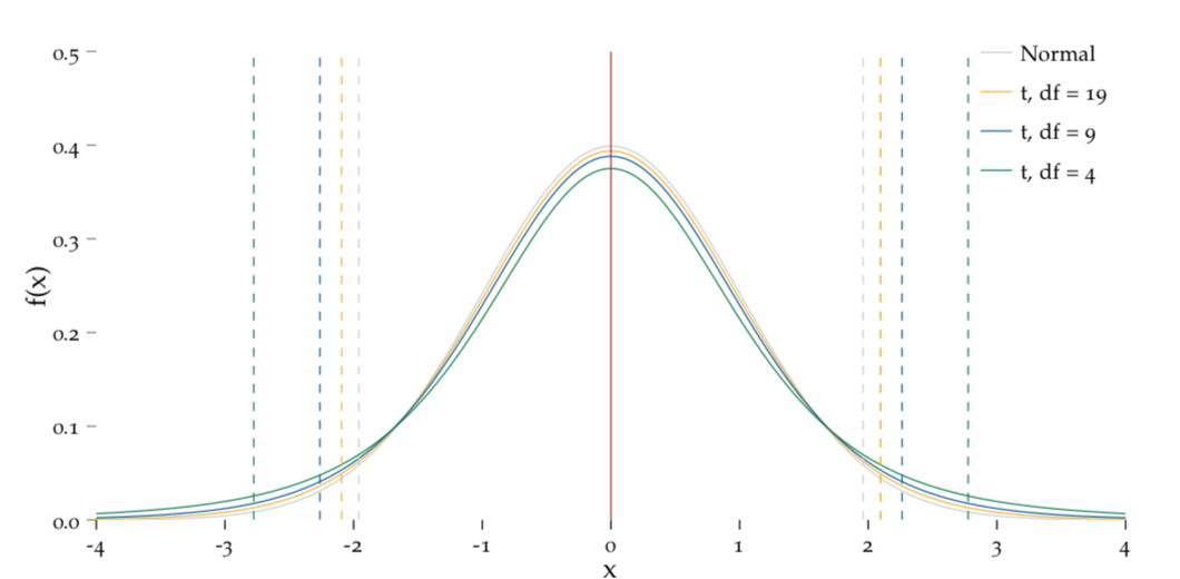
Figure 8.2: The shape of the t-distribution is determined by the degrees of freedom.

The dashed lines mark the interval covering 95% of the potential X values, centered around $0$. We see that as the df increases, this interval shortens, and the $t$–distribution gets closer and closer to the standard Normal distribution.

The second point means that the shape of the $t$–distribution changes dependent on the sample size. From Figure 8.2, we note that the larger the degrees of freedom (i.e. the larger the sample size) the⁵⁰ more the $t$–distribution resembles the standard Normal distribution. This is due to the fact that the extra uncertainty we have from estimating instead of knowing $\sigma$ decreases with a bigger sample size. This extra uncertainty is what is responsible for the fatter tails of the $t$–distribution when we compare it to the standard Normal distribution. Apart from this slight change in distribution, everything we said so far about testing stays the same!

That was the good news, now the bad news: in a strict sense, we can use this nice $t$–distribution only if the variable of interest is Normally distributed in our population. So whenever we are planning to do a $t$–test we need to make sure this underlying assumption is met.⁵¹

Let’s explore what all the means using the web app: use the t-distribution web app to answer the following questions:

What are the boundaries of the central interval of the $t$–distribution that encompasses 95% probability if you have a sample size of $n=$5?:
What happens to these boundaries if $n$=10?

Going back to our Martian height example, we saw that the observed $t$–statistic is $t=(200 - 195)/1.9 = 2.64$ which is outside the interval [-2.26, 2.26]. This tells us once more that it is very unlikely that our assumption of Martian height being $195$ cm based on popular culture references was correct. However, we also see that accounting for the extra uncertaincy of not knowing $\sigma$, our result is not quite as clear cut as before, when we compared $(200 - 195)/1.9 = 2.64$ to the interval [-1.96, 1.96].

Given this new insight, would you now reject $H_0: \mu = 196$ cm? How did you come to this conclusion?

8.6 The ‘p–word’

At this stage we have shown in different ways that our popularly held belief that the true mean Martian height is 195 cm, is probably wrong. In particular, we have demonstrated that if this hypothesis were correct, it would be less than 5% likely to observe 10 Martians that on average have a height of $\bar{x} = 200$. While this amount of information might satisfy some people, most researchers are more curious and want to know more: what does less than 5% mean? Exactly how likely is it then?

The answer to this question can actually be quite easily obtained by looking at the $t$–distribution again. Just as we can find out that all values outside [-2.26, 2.26] are less than 5% likely, we could try to find out how likely it is to observe values outside the interval [$-2.64, 2.64$]. This probability would tell us, how likely it is to observe a sample with the same or more extreme signal to noise ratio, i.e. the same or bigger standardised deviation between the observed mean $\bar{x}$ and the hypothesized value $\mu_0$. This is what the $p$–value is in our case!!

Use the web app to do exactly this.

More generally, the $p$–value is defined as

The $p$–value is the probability of observing data that show at least as much deviation from the null hypothesis (i.e. that are at least as unlikely to have been observed by chance) as the data we have at hand, assuming that the null hypothesis were true.

This definition explains why small $p$–values result in a rejection of the null hypothesis. It may sound a bit clumpsy though so let’s reiterate reiterate things using an example close to home.

8.7 Understanding ‘p–values’

Let us suppose that it’s late Autumn, so the weather is on the brink of getting very cold. We have a fancy new sweater that we really want to wear, but if it’s too cold, we’ll have to settle with our ugly old winter jacket. To tackle this serious problem in an appropriate way, we formulate the null hypothesis that it’s very cold outside, e.g. $H_0: \mu\leq10$ celsius.⁵² Since we’re scientists, we want to probe this hypothesis by collecting some data. In this case, we look out the window and note what people are wearing. The $p$–value that we then mentally obtain relates what we observe with what we expect under the null hypothesis via the question

If the null hypothesis, $H_0: \mu\leq10$ celsius, were true, how likely is it to observe what I observe?

Clearly, the likelihood of seeing people in summer clothes when it’s $\leq10$ celsius is not very large. Therefore, the more people we see wearing T–shirts, the bigger the deviation between our data and what we expect under $H_0$, the smaller the $p$–value, and the bigger our inclination to reject $H_0$ and leave our ugly jacket at home when we leave the house!

% So imagine, we saw many people in T–shirts. This would not be very consistent with $H_0$, so we would be inclined to reject it and leave our ugly jacket at home when we leave the house. However, and this is an important point, there is still a chance that we were just really unlucky when we collected the data and accidentally the people that we observed just happened to be wearing summer clothes for some reason despite it being very cold. Admittedly, that’s not very likely, but the probability of accidently rejecting the null hypothesis is not zero! We’ll talk about this kind of mistake in a bit. First, let’s reiterate what we learned in this section:

8.8 The significance level, $\alpha$

If the $p$–value is small, we are inclined to reject the null hypothesis. But how small does it need to be?! Everyone knows that the usual strategy is to reject the null hypothesis if the $p$–value is less than 0.05. Sticking to this procedure would mean that we accept at most a 5% chance of accidentally rejecting the $H_0$ despite it being true. However, it is important to point out that 0.05 is not a God–given magic number, and just choosing it out of convention does not make much sense. Instead, we need to make up our own mind as to how important it is to not accidentally reject $H_0$ in our particular study. We therefore need to define a (study–specific) threshold for the $p$–value beyond which we will reject the $H_0$! This threshold is called the significance level and is commonly denoted by $\alpha$.

To understand $\alpha$, let’s return to our sweater weather example. Here, we would choose $\alpha$ depending on how much we hate being cold. If we don’t mind being cold, then our strategy could be to set a quite liberal (i.e. large) significance level like $\alpha = 0.2$. With this, we don’t require too much evidence against $H_0$ before we reject it, a $p$–value $< 0.2$ would be enough. However, if we absolutely detest being cold, then we are not very inclined to reject the $H_0$. In this case, our strategy would be to select a very stringent significance level, e.g. $\alpha = 0.001$, which means we will only reject $H_0$ if we saw lots of people in $T$–shirts and the evidence against it being cold is absolutely compelling.

% Similarly, if you make a discovery in your research that would make it necessary to re-write the textbooks you’d better be really sure about your results before you submit them to Nature (small $\alpha$). If your results are only supposed to be the starting point for new experiments in your lab you don’t need to be quite so certain that they are based on something real (large $\alpha$)!

Similarly, in the Martian height example, the $p$–value threshold we choose beyond which we reject the hypothesis $H_0: \mu=195$ cm should depend on how bad an accidental rejection would be. To stick with our slightly made up explanations: if the person who proposed this hypothesis in the first place was a famous and well-respected editor of many important journals in your field, then you want to be really sure before you claim that he’s wrong. In this case, you’d choose a stringent significance level $\alpha$ and only reject the null hypothesis for very small $p$-values, i.e. when the evidence against it in your data is very strong.

By the way, rejecting the null hypothesis is what’s commonly called ‘the test was significant’. The long (and more correct) version of saying this would be to say

The data showed statistically significant deviation from the null hypothesis of xxx at the yyy % level.⁵³

8.9 Summary thus far

We have covered quite a bit of material regarding hypothesis testing already. Before we move on, let’s take a little break and summarise what we’ve learned so far.

Test statistics tell us something about the size of the observed difference between the data and the null hypothesis (i.e. the signal) relative to the uncertainty in the sample (i.e. the noise). The farther away our observations are from $H_0$, the larger (in absolute terms) the value of the test statistic will be, i.e. a large absolute value of the test statistic gives us a hint that the deviance between the data and the null hypothesis is due to some systematic pattern and not just due to unlucky sampling. A standardised way to make a judgement about this is the $p$–value: the larger the value of the test statistic, the more evidence against $H_0$ is contained in the data and the smaller the $p$–value. If it is smaller than a certain threshold $\alpha$, the null hypothesis is rejected based on the data. The significance level, $\alpha$, thus controls the probability that you accidently reject $H_0$, i.e. a false positive result. We’ll return to this soon.

8.10 One and two–sided tests

In hypothesis testing, it’s not only important to specify the null hypothesis, $H_0$, but also the departure from $H_0$, i.e. the alternative hypothesis $H_1$ which can be thought of as the opposite of $H_0$. Recall that $H_0$ usually describes the state that is not interesting, i.e. the state of boredom. Conversely, $H_1$ matches our a priori desire of what would be interesting to discover in the data. Taken together, $H_0$ and $H_1$ are called the test problem, and as we’ll see now, it can come in different versions.

In the sweater weather example, temperatures $\leq10$ celsius weren’t interesting, since we couldn’t wear our sweater. Therefore, the desirable state is the case where the temperature exceeds $10$ celsius. The entire test problem can be thus be formalised as

\[H_0: T \leq 10celsius \quad \quad \mbox{vs.} \quad \quad H_1: T > 10 celsius.\]

In the Martian height example, any departure from $H_0$ is interesting, we have no a priori reason to be more excited about Martians to be taller or shorter than the hypothesised value $195$ cm. Thus, the test problem can be formalised as

\[ H_0: \mu = 195cm \quad \quad \mbox{vs} \quad \quad H_1: \mu \neq 195cm.\]

These cases demonstrate the difference between one–sided and two–sided test problems. In total, there are three possible scenarios that are summarised in Table ScenarioDescriptions.

Table 8.1: Three scenarios in hypothesis testing and two types of tests: two–sided and one–sided.
Scenario	$H_0$	$H_1$	a priori expectations	Type
1	$\mu=\mu_0$	$\mu\neq\mu_0$	$\bar{x}$ differs from $\mu_0$	two–sided
2	$\mu\geq\mu_0$	$\mu<\mu_0$	$\bar{x}$ is less than $\mu_0$	one–sided
3	$\mu\leq\mu_0$	$\mu>\mu_0$	$\bar{x}$ is greater than $\mu_0$	one–sided

Exercise Can you think of a weather problem that is one–sided but in the other direction?

Exercise Can you think of a two–sided weather problem?

Exercise What are one– and two–sided scenarios in your own research?

The distinction between one– and two–sided test problems is important because it influences the $p$–value. Too see this, let’s return to the Martian height example and consider all 3 scenarios listed in Table ??. The corresponding graphical explanations are shown in Figure 8.3.

8.10.1 Scenario 1: two–sided tests, $H_0: \mu=\mu_0$

We already defined our Martian height situation as being two–sided. That means we are looking at the test problem:

\[H_0: \mu = 195 cm \quad \quad \mbox{vs.} \quad \quad H_1: \mu \neq 195 cm.\]

We observed that $\bar{x}>\mu_0$ (i.e. $200$ cm > $195$ cm, i.e. look at the right–hand side of the top row of Figure 8.3.). Our standardised way of assessing the deviance between the sample and the null hypothesis gives us the test statistic

\[t=(\bar{x}-\mu_0)/SEM = (200-195)/1.9 = 2.64.\]

The dashed red line shows the position of this value on the corresponding null distribution, $t_{9}$. We find that the area under the curve to the right of 2.64 (shown in red) is very small. It corresponds to $0.0135$, i.e. if the null hypothesis were true there is only a 1.35% chance to observe a sample of 10 Martians with a mean height of 200 cm or larger (i.e. more extreme). But wait! In the two–sided case, this is only half of the story. The term more extreme refers to deviations from $H_0$ to either side. Therefore, we also need to consider the area under the curve to the left of -2.64 which by the way would correspond to an observed $\bar{x}$ of $190$ cm as

\[t=(190- 195)/ 1.9 = -2.64.\] Since our test is two–sided, $\bar{x} = 190$ cm provides as much evidence against $H_0$ as $\bar{x} = 200$ cm. Due to the symmetry of the $t$–distribution we know that the area under the curve to the left of -2.64 is also $0.0135$, i.e. if $H_0$ were true, there is only a 1.35% chance to observe 10 Martians with a mean height of $190$ cm or smaller (i.e. more extreme). Taken together, this means that there is a $2.7$% chance to observe a sample that provides at least as much evidence against $H_0$ as the one we observed. This is exactly the $p$–value we’re interested in in the two–sided scenario. We add up the area under the curve beyond the t-statistic from both directions. As $p < 0.05$, we reject the null hypothesis at the chosen significance level $\alpha = 0.05$.

Important point number 1: In the two–sided case, exactly the same considerations hold true if we had observed $\bar{x} = 190$ cm which corresponds to the left–hand side of the top row of Figure 8.3.
Important point number 2: Note the position of the dashed blue lines. These the values of the test statistic would result exactly in a $p$–value of that matches the chosen significance level, i.e. $p = 0.05$ in our case. They are called the critical values for $\alpha = 0.05$ because any test statistic beyond these values would yield a significant result, i.e. result a $p$–value less than $0.05$.

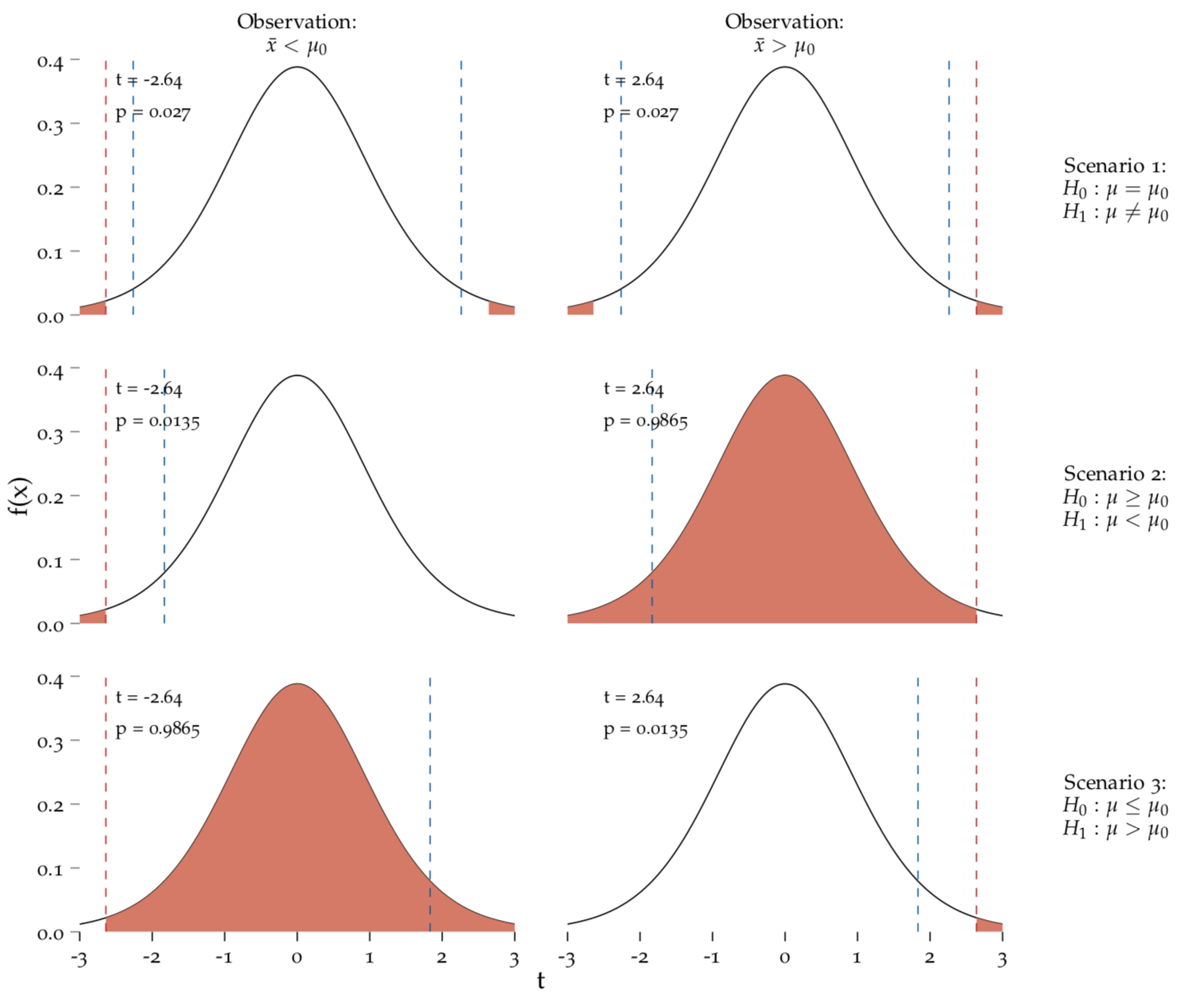
Figure 8.3: Two–sided and one–sided tests.

Three scenarios and two possible outcomes of statistical tests. Each scenario is plotted on a $t_{9}$ distribution with critical values at $\alpha=0.05$ depicted with dashed blue lines. The $p$–value corresponds to the red area.

8.10.2 Scenario 2: One–sided tests, $H_0: \mu\geq\mu_0$

If we had some a priori reason why it only would be interesting if the mean Martian height is smaller than what is currently believed, we would have formulated our test problem as

\[H_0: \mu \geq 195 cm \quad \quad \mbox{vs.} \quad \quad H_1: \mu < 195 cm.\]

This case is presented in the middle row of Figure 8.3. Again, the right panel shows our current situation, where $\bar{x}>\mu_0$ (i.e. $200$ cm > $195$ cm). The $t$–statistic, the dashed red line, is the same as before: $t=2.64$. However, due to the different nature of the test problem, this situation results in a very large $p$–value compared to the two–sided test: $p = 0.9866$, which is reflected in the red-shaded area under the curve to the left of our $t$-score. This is because our observation, $\bar{x}>\mu_0$, is perfectly in agreement with $H_0: \mu\geq\mu_0$! There is no evidence in the data against the null hypothesis. Unfortunately, this is corresponds to the situation that is not of interest for us.

Exercise Given that the $p$–value for the two-sided test is $0.027$, can you write the formula for this $p$–value. Remember that the entire area under the curve sums up to one.

Conversly, if $\bar{x} = 190$ cm, i.e. $\bar{x}<\mu_0$, the situation is reversed as depicted in the left panel of the middle row of 8.3. The $t$–statistic is large and the $p$–value is tiny: $0.0134$, because our data are not in agreement with $H_0$. It would be very unlikely to observe $\bar{x} = 190$ cm in a sample of 10 Martians if $H_0: \mu \geq 195$ cm were true.

⁵⁴ Given that the $p$–value for the previous observation case $\bar{x}>\mu_0$, is $p = 0.9866$, what is the formula for this $p$–value? What is the relationship of this $p$–value to the $p$–value we observed for the two-sided test, i.e. $p=0.027$?

Before we move on the scenario 3, also take a look at the position of the critical values, i.e. the blue lines. In a one-sided test, there’s only one critical value but as before it’s positioned on the side of the curve in accordance with $H_1$, i.e. in a region where we’d reject $H_0$.

Exercise Why are the critical values in the one–sided test closer to zero than int he two–sided scenario?

8.10.3 Scenario 3: One–sided tests, $H_0: \mu\leq\mu_0$

This situation is exactly the same as in scenario 2, except that everything is reversed. In this situation, we have the test problem

\[ H_0: \mu \leq 195 \quad \quad \mbox{vs.} \quad \quad H_1: \mu > 195,\]

which is depicted as scenario 3 in the bottom row of Figure 8.3.

Notice that the critical values, the dashed blue lines, and the area under the curve contributing to the $p$–value are on the right side of the curve. This reflects the direction of the test, since only high $t$–statistics will result in a “significant” result. Our current situation, $\bar{x}>\mu_0$, shown in the right panel, speaks against $H_0$ and results in a small $p$-value. This is exactly the same as the left panel of scenario 2, just on the opposite side! The converse outcome, $\bar{x}<\mu_0$, shown in the left panel, is in agreement with $H_0$ and results in a very large $p$–value. This is exactly the same as the right panel of scenario 2, just on the opposite side!

8.11 Errors in hypothesis testing

As mentioned above, the significance level $\alpha$ controls the probability to accidently reject $H_0$. This is one of two types of error that can occur in hypothesis testing. The two error types can have different names depending on the text book you look at which can sometimes be a source of confusion, so let’s spell them out in detail:

Type I error⁵⁵ also known as the $\alpha$–error, corresponds to rejecting the null hypothesis $H_0$ although it is true. Type I errors are referred to as false positives.

Type II error also known as the $\beta$–error, corresponds to not rejecting the null hypothesis $H_0$ although it is false. Type II errors are referred to as false negatives.

The two error types above are flip–sides of each other. Actually, they are two out of four possible outcomes that we can get in hypothesis testing as shown in Figure 8.4.

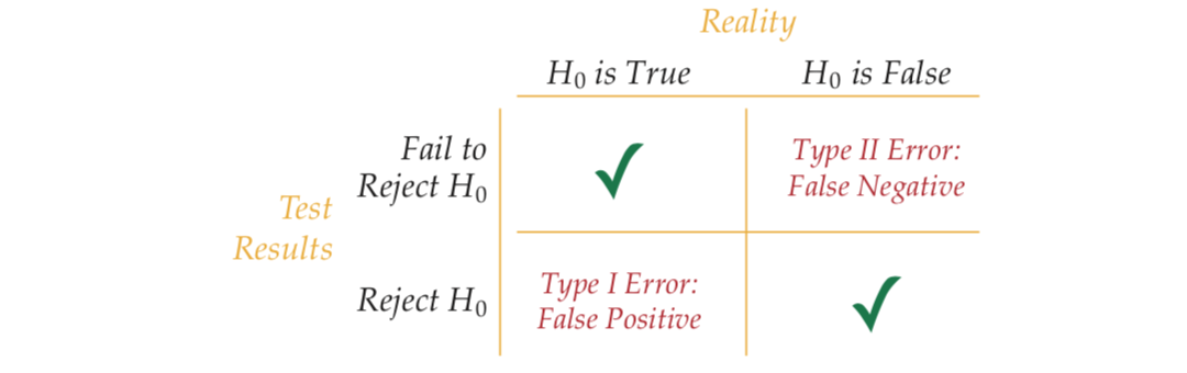
Figure 8.4: The four possible outcomes of hypotheses testing – there are two ways to get it right and two possible pitfalls.

To understand the two types of error, we’ll return to the sweater weather example. Here, the null hypothesis is $H_0: \mu\leq10$ celsius, i.e. the state we hope to disprove. The null hypothesis can be either true or false, this is the underlying reality that is unknown to us and that we want to find out about by collecting the data. Based on data, we get a test result, i.e. we can either reject the null hypothesis or not. In total, we get the four outcomes shown in Figure @ref(fig:fouroptions_sweater).

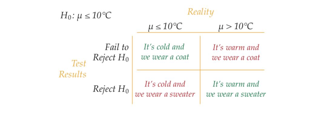
The four types of outcomes in the sweater weather example. The desired options are show in green, and our most favourite is the true positive where it indeed is warm and we leave the ugly coat inside.

(#fig:fouroptions_sweater)The four types of outcomes in the sweater weather example. The desired options are show in green, and our most favourite is the true positive where it indeed is warm and we leave the ugly coat inside.

⁵⁶

A false positive here would be that we accidently reject $H_0$ based on the data, i.e. we think we have seen a sufficient number of people in summer clothes to decide that it’s probably not so cold, so we walk outside with a sweater and get a bad surprise because in fact $H_0$ is true and we and up freezing.
A true positive is our preferred outcome, i.e. we reject $H_0$ wear our sweater and it’s nice Autumn weather.
A true negative would be OK as well, it is the situation where we don’t find enough evidence against the hypothesis that it’s cold and decide to wear a coat when indeed it is cold. We have to wear the ugly coat but at least we are not freezing.
A false negative here would be the situation where we reject $H_0$ based on our data, wear the ugly coat although actually it’s warm outside and we and up sweating all day.

⁵⁷

In the sweater weather example, both types of error are not desirable because you end up either freezing or sweating. So how do we deal with the errors?! In hypothesis testing, the error that you actively deal with is the type I error, by choosing your significance level $\alpha$. Adhering to your choice will make sure that the probability of a type I error is not going to be bigger than $\alpha$. However, if you choose a small $\alpha$, you need to be aware that this increases the chance of a type II error! ?? So there is a trade–off between them.

Exercise In the sweater weather example, what would happen if you chose a very stringent (i.e. small) significance level?

8.12 Power

There is only one more term that we need to explain before you know the most relevant vocabulary in hypothesis testing, and this is power. As you the name suggests, power is something that we want in a test, so let’s talk about how we can get lots of it! So far we have mainly talked about type I error, i.e. the error that corresponds to the left–hand side of Figure ?? when $H_0$ is true. But what happens on the other side, when $H_0$ is false? Either we incorrectly fail to reject $H_0$ (type II error) or we correctly reject $H_0$. The convention is to denote the probability of a type II error with $\beta$ which directly leads to a probability of $1-\beta$ for a correct rejection of $H_0$ – this is the famous power of a test:

Statistical power is the probability of rejecting a false null hypothesis $H_0$. This corresponds to the probability of a true positive. In other words, it is the ability to detect an effect when it is there.

So for a given test, how do we determine the probability of the type II error, and thus the power? Is there is procedure to control for it in a way that is similar to setting a significance level which sets an upper limit on the probability of conducting a type I error? Unfortunately the answer is no – $\beta$ cannot be controlled for directly. It is indirectly determined by three factors: the significant level $\alpha$, the effect size of interest, and the sample size.

In the following, we will demonstrate these dependencies using the Martian height example, and to make it easier to understand we’ll just stick to the one–sided test problem \[ H_0: \mu \leq 195cm \quad \quad \mbox{vs} \quad \quad H_1: \mu > 195cm.\] The top panel of Figure 8.5 shows the null distribution for this test problem.⁵⁸ It is centered around the hypothesised value. The additional panels below correspond to different versions of a situation where the alternative hypothesis is true, namely to $\mu = 197$ cm, $\mu = 200$ cm, and $\mu = 203$ cm, respectively. In these situations, we would like to reject the null hypothesis.

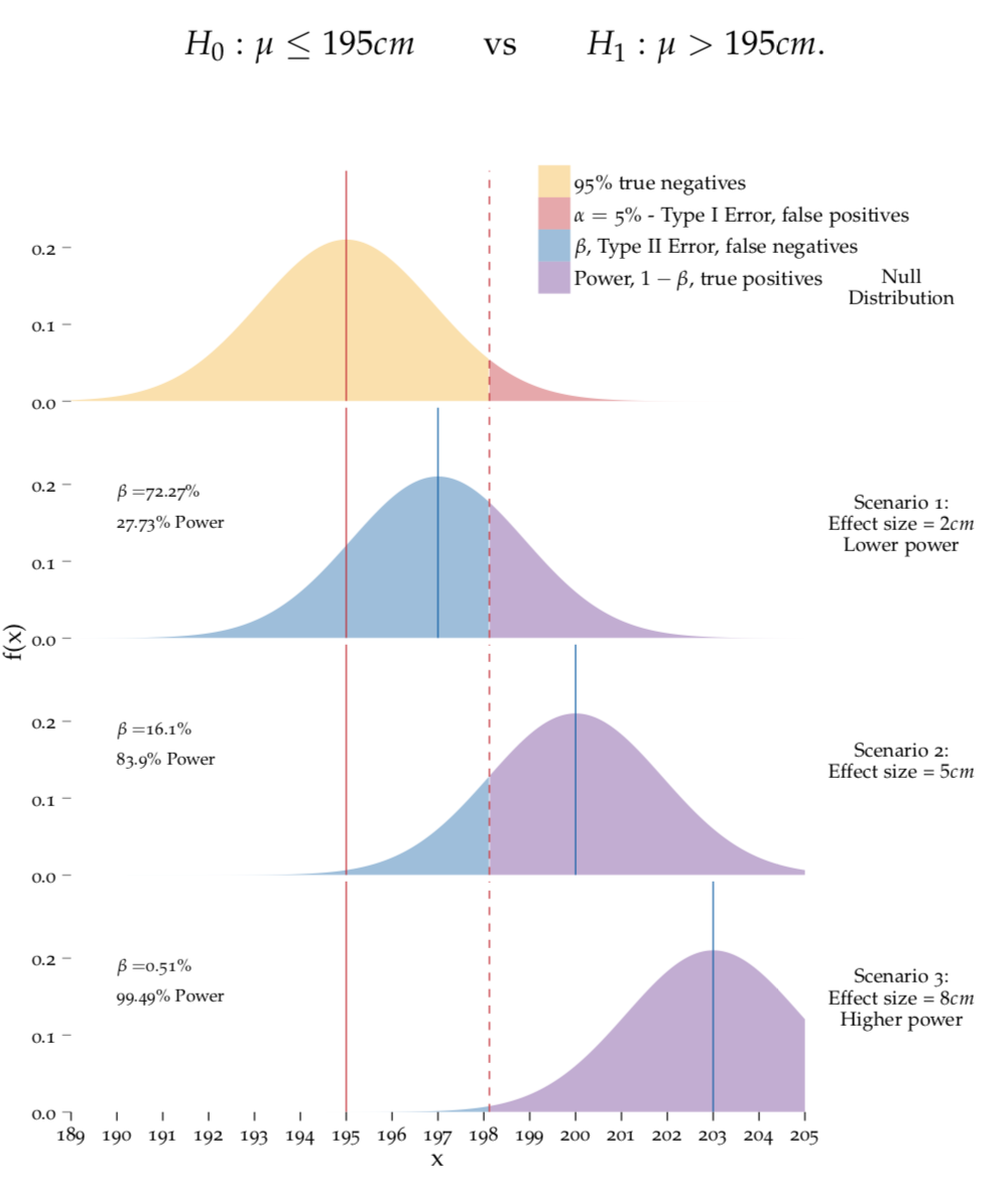
Figure 8.5: Calculating power.

top panel: The null distribution is what we expect to observe if the null hypothesis were true, it is therefore centered around the hypothesised $\mu$ (solid red line). The dotted red line marks the critial value, which is determined by $\alpha$. lower panels: The distributions depict what we expect to observe in different situations where the alternative hypothesis is true. Note that these situations exhibit a sequentially increasing departure from $H_0$. In each case, the area of the region beyond the critical value corresponds the probability of obtaining a true positive result, i.e. the power of our test under these circumstances.

8.12.1 Dependence on the significance level, $\alpha$

In Figure PowerOneSided, the significance level is chosen as $\alpha = 0.05$. This choice determines the critical value that is displayed by the dashed line. Let’s call this $x_{crit}$. This critical value separates the null distribution (top panel) into two parts, yellow and red. The yellow part makes up 95% of the area under the curve. Conversely, the red part makes up 5% of the area under the curve. Whether or not we reject the null hypothesis, depends on the observed $\bar{x}$. We reject if $\bar{x} > x_{crit}$ which – by design of the critical value – happends in only 5% of the cases if the null hypothesis is true.

Now consider the bottom panels which depict situations where $H_1$ is true and we want to reject the null hypothesis. The probability of this is shown in purple in these situations. It corresponds to the power respective power. So what happens to the power if we change $\alpha$? Imagine, we decrease it to say $\alpha = 0.01$. This moves the critical value to the right, and will decrease the area of the purple part in all bottom panels! This is the trade–off between type I and type II error that we previously talked about. If we decrease $\alpha$, we decrease the probability of a type I error because the evidence in the data against the $H_0$ needs to be very large before we reject $H_0$. However, this also means that the probability to not rejecting $H_0$, although it is false, can be quite big.

8.12.2 Dependence on the effect size

The effect size is defined as the departure of reality from the null hypothesis. The bottom panels of Figure 8.5 therefore show three different effect sizes, namely 2 cm, 5 cm, and 8 cm, respectively. We can see that the power (the purple area under the curves) changes depending on the position of the bottom curve which in turn is governed by the effect size. The bigger the effect size, the farther the distribution of $\bar{X}$ moves away from the null distribution and power increases. In other words, the bigger the true $\mu$, the more likely it is to observe a $\bar{x}>x_{crit}$ in which case we reject $H_0$.

To demonstrate this further, imagine the extreme case where $\mu = 195.0001cm$. Although we are still in the case where we’d like to reject the null hypothesesis, the signal $\mu - \mu_0$ is very small, so even without math we intuitively know that this effect will be hard to detect. Visually, we can also confirm this intuition by imagining the lower panel curves in Figure 8.5 moving to the left until they are centered around $\mu = 195.0001cm$. In this case the blue area will grow a lot and with it the probabilty to conduct a type II error. Conversely the power decreases!

This raises the question: if power changes depending on the position of the true $\mu$ (which is unknown to us!!), how can it be calculated? It can’t unfortunately, but to rescue the situation, we use a worst–case–scenario where we consider the minimal effect size that we would like to be able to detect and caclulate the maximally possible power. In our example, imagine that we only consider our finding exciting if the true Martian mean height is at least $2$ cm greater than $\mu_0=195$ cm. This means that we would carry out our power calcuations based on Scenario 1 where $\mu = 197$ cm.

8.12.3 Dependence on the sample size

Let’s stay with the Scenario 1 in Figure 8.5, where the effect size is 2 cm and power is $0.28$. What if we are not happy with this value and we would like to have a greater chance to detect a signal of 2 cm with our test? Say we would like to a power of $0.84$ instead (which is the power of Scenario 2 where the effect size is 5 cm)! This is where sample size comes in. To see this, remember our good old friend the CLT - the $SEM$ decreases as sample size increases.⁵⁹ This ensures that you can estimate $\mu$ with greater precision, and in terms of Figure 8.5 it means that the overlap between the top and the bottom curves decreases although the effect size (i.e. the distance between the centers of the curves) stays the same.

In Figure 8.5, we calculated the shown power values using a sample size of $n=10$. To achieve the desired power $0.84$ for detecting an effect size of 2 cm, we’d need to have a sample size of 62! This is shown in Figure 8.6. Note how high and narrow the distributions are which reduces the overlap between the two curves. Also notice that the critical value has shifted.

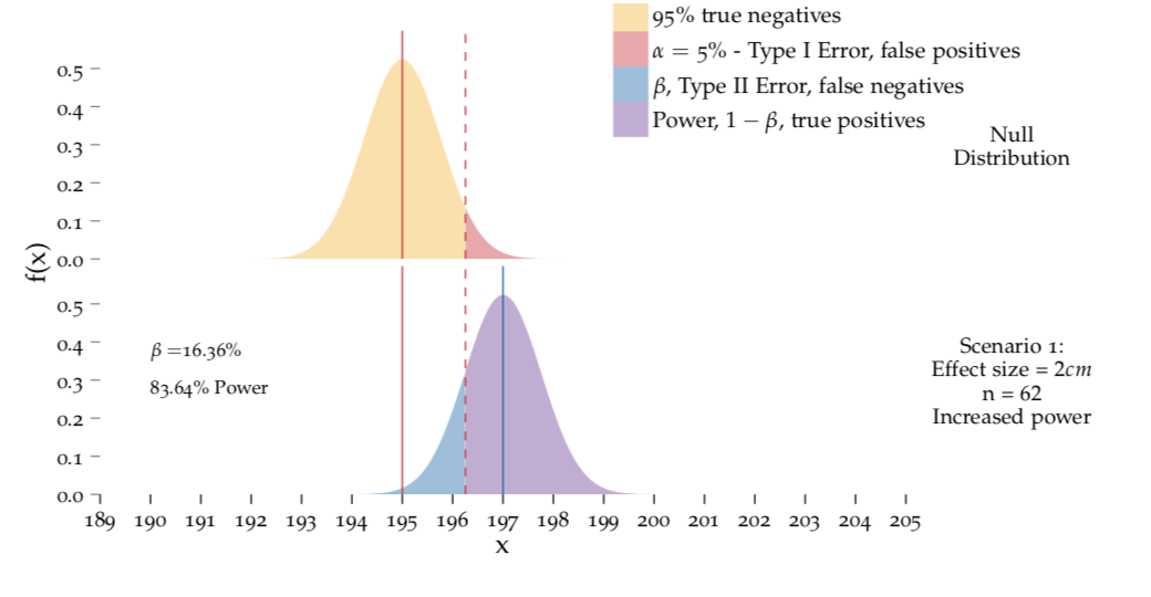
Figure 8.6: Calculating power.

top: The null distribution with $n = 62$. bottom: The disribution of $\bar{X}$ with an effect size of 2 cm, i.e. $\mu = 197$ cm. Compared to Figure 8.5 the curves are very narrow and don’t overlap as much which increases the power.

Exercise Given that the sample size influences power via the $SEM$, can you derive how population variance influences power?

In summary, the coloured partition of the curves in Figures 8.5 and 8.6 is dependent on four factors. Figure ?? gives an overview about the effect of these factors on the power!

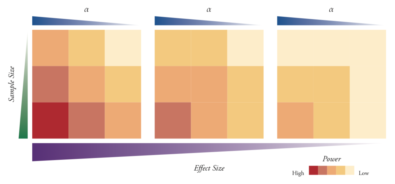
Figure 8.7: Calculating power.

The power of a statistical test is dependent on four factors: the sample size, the population variance, the significance level, and the effect size under investigation. For a given significance level, the highest power is achieved with a large sample size, a small population variance and large effect sizes. Here, the effect of significance level, effect size and sample size are depicted for a fixed value of the population variance. A qualitative colour scale depicting power under different conditions.

8.13 Sample size calculation in hypothesis testing

So how can we determine the sample size we need to detect a certain effect size with a certain power? For different tests, the formula comes with different flavours. However, in general, we can use the following recipe:

Choose the significance level, i.e. the maximum type I error rate that you’re willing to accept in your study.
Choose the minimal effect size that you are interested in.
Identify the sources of variation in your experiment and make a best-guess of their magnitude, either from previous experiments or from literature.
Choose the power that you want your experiment to have.
Calculate the sample size that would allow you to achieve this power, given the first three points.

8.14 Some words of caution

Within this book, this chapter contains the toughest material – well done for seeing it through! Things will fall into place from now on and will become easier to understand. Before we move on though, we’d like to draw your attention to three more things!

8.14.1 What makes a Good Hypothesis?

Usually, you don’t just collect data for fun, but with a certain question in mind. Good hypotheses, in the context of hypothesis testing, are testable questions that are derived from your research question. Sometimes the research question needs to be broken down so that it can be written (with a formula) in terms of a null hypothesis and a suitable alternative. That’s a shame but if you manage, your test results will be meaningful!

8.14.2 Statistical versus practical significance

We saw that the magnitude of a $p$–value depends on several factors, and not all of them tell you anything about the practical significance of your results.⁶⁰

In a way, statisticians have hijacked the ordinary meaning of the word significance, which implies important and practical relevance. Statisticians have given the word significance its own meaning. Some not very statistically inclined people may not realise this and may get excited about a statistically significant finding, when actually:

The technical term statistically significant relates to the mere existence of an effect, not about the size. To give yourself and the readers of your publications the chance to also assess the practical significance of your results ALWAYS PROVIDE A CONFIDENCE INTERVAL.

8.14.3 Interpreting non-significant results

What’s the right way of interpreting a non-significant $p$–value⁶¹? In some papers you can read something like ‘we accept the null hypothesis’. If this statement is based on a statistical hypothesis test, it is actually flawed! As we mentioned before, a non-significant $p$–value merely shows that you cannot rule out the null hypothesis. Based on the duality between confidence intervals and hypothesis testing that we covered in section ??, however, we know that there are many values that we cannot rule out, i.e. all values inside your confidence interval! So we cannot accept just one of them!

Knowing this will also help you understand why the null hypothesis is usually chosen as the state of boredom that you want to reject. It is because you cannot prove anything that you want to see, all you can do is to reject the stuff that is of no interest for you!

There are two lessons to be learned from this: - Never state that the null hypothesis is true, or that you accept the null hypothesis. - Never quote a $p$–value without a confidence interval.

Whenever we talk about the CLT, we implicitly assume that we are in the situation where the sample size $n$ is big enough so that the it holds true!↩
In hypothesis testing, we pretend that $H_0$ is true, and then look how likely it is that we observe the given data under this premise! In other words, we find out how much our data support the null hypothesis.↩
All values $\mu_0$ that are not inside the 95% confidence interval can be rejected with 95% confidence.↩
This is is a general statement! Here you can choose the confidence level as you like. If you are happy with the idea to accidentally reject $H_0$ even if it’s true with a chance of $\alpha$%, then choose a ($1-\alpha$)% confidence interval. More on $\alpha$ later.↩
Recall that N(0,1) means the standard Normal distribution, with a $\mu$ of 0 and a $\sigma^2$ of 1. The notation $\stackrel{H_0}{\sim}$ is a quick and lazy way of saying ‘distributed under the null hypothesis’. This formula tells us that $(\bar{X} - \mu_0)/SEM$ has a standard Normal distribution if $H_0: \mu = \mu_0$ is true.↩
The signal–to–noise ratio in the current context is essentially the same thing as a $Z$–score!!!↩
And this is because with $Z$–scores, the limit for a 95% certainty will always be 1.96.↩
This is true for any hypothesis test, including all the practical examples that we’ll talk about in the next chapter!↩
Another way of understanding this is to think about being penalised for having a small sample size. Smaller sample sizes equate to fatter tails and wider 95% probability ranges.↩
This is quite important when you have a small sample size. With big sample sizes, we’re back to the CLT and we can revert to the Normal distribution! We’ll talk more about underlying assumptions when we get to non–parametric tests.↩
Note that we use the state that we want to reject (it being cold) as the null hypothesis. This is a convention in hypothesis testing which also has a mathematical reason as we’ll see later.↩
Obviously replace xxx with your specific null hypothesis and yyy with your chosen significance level $\alpha$.↩
A convenient way to remember which part of the curve will contribute to the $p$–value is to look at $H_1$. For $H_1: \mu\neq\mu_0$, it’s the area beyond the $t$–statistic in both directions. For $H_1: \mu<\mu_0$, it’s always that which is lower than the $t$–statistic.↩
Note the confusing use of the term ‘positive’ here. A positive result is we reject the null hypothesis. This is because usually $H_0$ is the state of boredom you want to reject. By the same token, a negative result is not being able to reject the null hypothesis – boring!↩
A general comment: Note that we deliberately never say that we prove $H_0$. In hypothesis testing, we either reject or cannot reject the null hypothesis $H_0$, but we never prove it. Why is that? We give the answer to this at the end of the chapter!↩
In a research setting, a false positive is akin to thinking you have a fantastic new result, when you actually don’t!↩
This is just a repetition of Scenario 3 from Figure 8.3, but we’re going to make things easier by simply using the Normal distribution.↩
You can see this in very large studies, where tiny effects are considered significant, primarily because the sample size is really big.↩
If the sample size is large, then it is possible to find very tiny deviations from the null hypothesis in your data that may not be of any practical importance.↩
Actually, the term ‘a non-significant $p$–value’ doesn’t make much sense if we are strict! What people mean when they say that is a $p$–value that exceeds the chosen significance level $\alpha$, which in most cases corresponds to $p > 0.05$. As you know now, however, $\alpha$ can in principle vary and should always be included in the sentence when you talk about statistical significance.↩

Scenario	\(H_0\)	\(H_1\)	a priori expectations	Type
1	\(\mu=\mu_0\)	\(\mu\neq\mu_0\)	\(\bar{x}\) differs from \(\mu_0\)	two–sided
2	\(\mu\geq\mu_0\)	\(\mu<\mu_0\)	\(\bar{x}\) is less than \(\mu_0\)	one–sided
3	\(\mu\leq\mu_0\)	\(\mu>\mu_0\)	\(\bar{x}\) is greater than \(\mu_0\)	one–sided

Statistical Literacy