Chapter 4 Case Study: Plant Growth

Exercise 4.1 (R Syntax) Start building a script by entering the commands into the text editor and then executing them in the console (press ctrl + enter). Commands will appear after the > sign.

PlantGrowth

PlantGrowth is a built-in data-set of plant dry-weight. If you execute PlantGrowth in the console, you’ll see the entire data-set. The group column is a categorical variable, describing if dry-weight was measured under control (ctrl) or one of two different treatment (trt1 and trt2) conditions. This experimental set-up is probably familiar to you, even if you are not studying plant growth.

We already have access to the data set, in the form of a data frame. To make it easier to print to the screen, we’re going to convert it to a tibble.

PlantGrowth <- as_tibble(PlantGrowth)

In many situations in statistics, categorical variables are called factors. Within a factor, each category, or group, is called a level. We can find out how many levels we have and what they are by using the nlevels() and levels() functions on the growth column:

nlevels(PlantGrowth$group)

# [1] 3

levels(PlantGrowth$group)

# [1] "ctrl" "trt1" "trt2"

Factors are very convenient because we can use them to split other columns. This is a very simple and powerful technique for handling data. To get a sense of the data’s distribution, we can draw a variety of plots, sorting each weight value according to the levels of the growth factor (i.e. the three growth conditions). The result is displayed in figure ??.

R specializes in handling and visualising data, so making the boxplot is straight-forward in base R. However, there are many new packages which have made things easier and more consistent, like ggplot2, which is included in the tidyverse suite. It offers fine control of making elegent statistical plots.

In the ggplot() function below, weight is mapped on the x scale, and weight is mapped onto the y scale. Collocualy, we would way, “weight against group”, or “weight as described by group”:

p <- ggplot(PlantGrowth, aes(group, weight))

Here is our box plot

p +
  geom_boxplot()

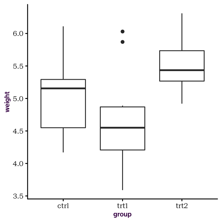
Figure 4.1: A box plot

p +
  geom_jitter(width = 0.2, shape = 16, alpha = 0.75) +
  stat_summary(fun.data = mean_sdl, fun.args = list(mult = 1), col = "red")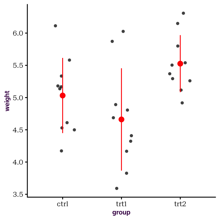

Figure 4.2: Summary statistics and raw values

We can get descriptive statistics on all the values in the weight column,

mean(PlantGrowth$weight)

# [1] 5.073

but group-wise statistics are more appropriate. You can imagine that statisticians have been doing such things for a long time. Let’s use some functions that come with the dplyr package, also included in the tidyverse suite.⁶

PlantGrowth %>%
  group_by(group) %>%
  summarise(avg = mean(weight),
            stdev = sd(weight))

# # A tibble: 3 x 3
#   group   avg stdev
#   <fct> <dbl> <dbl>
# 1 ctrl   5.03 0.583
# 2 trt1   4.66 0.794
# 3 trt2   5.53 0.443

As you can see from the example above, we can just keep adding to the summarise funcion – that’s really convenient!

In the above plot, stat_summary() calculated and plotted the group-wise mean and standard deviation for us. Now that we’ve calculated those values ourselves, let’s plot them directly. First, we need to save the output from above. If we just print it to the screen, there is no object to work on! Here, we’ll use a little trick that works well in combination with the %>% operator: the “reverse assign” operator ->. We only use this in the specific case of also using %>%.

PlantGrowth %>%
  group_by(group) %>%
  summarise(avg = mean(weight),
            stdev = sd(weight)) -> PlantGrowthSummary

Now I have an object that contains only my summary statistics. So let’s plot it!

ggplot(PlantGrowthSummary, aes(group, avg)) +
  geom_pointrange(aes(ymin = avg - stdev, ymax = avg + stdev))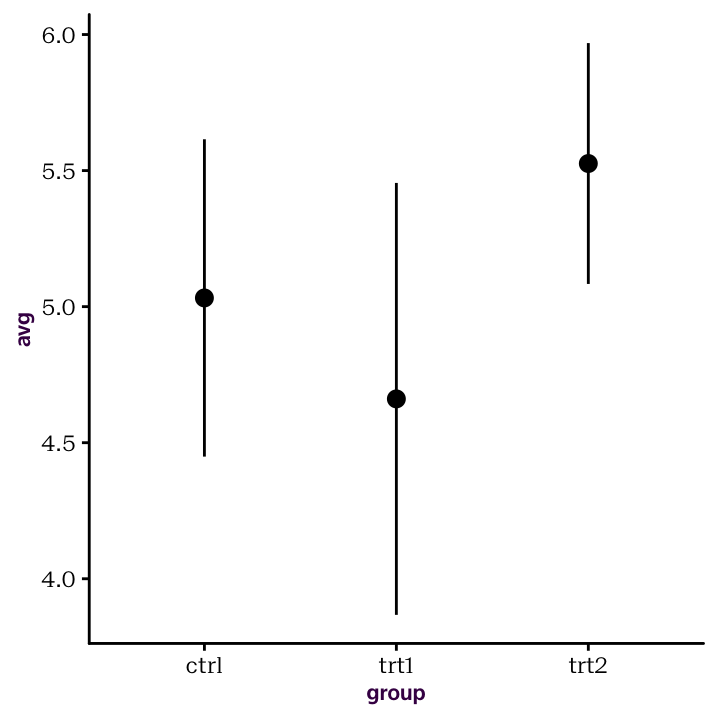

Figure 4.3: Summary statistics from their own, pre-calculated, data frame.

You can probably guess what the new parts of this plotting function are doing. I didn’t have to assign the base layers of the plot to an object, p above, because I just used it once and then it was finished.

Notice that PlantGrowthSummary only has three rows, since calculating the mean is an aggregration function, i.e. it aggergrates values to (typically) a single value. A Z-score is something quite different. This is a transformation, in which each value is transformed in some way (i.e. normalized). Again dplyr offers a solution:

PlantGrowth %>%
  group_by(group) %>%
  mutate(Z_score = scale(weight))

# # A tibble: 30 x 3
# # Groups:   group [3]
#    weight group Z_score
#     <dbl> <fct>   <dbl>
#  1   4.17 ctrl   -1.48 
#  2   5.58 ctrl    0.940
#  3   5.18 ctrl    0.254
#  4   6.11 ctrl    1.85 
#  5   4.5  ctrl   -0.912
#  6   4.61 ctrl   -0.724
#  7   5.17 ctrl    0.237
#  8   4.53 ctrl   -0.861
#  9   5.33 ctrl    0.511
# 10   5.14 ctrl    0.185
# # … with 20 more rows

Applying a linear model is also straight-forward. Consider a one-way ANOVA:

Plant.lm <- lm(weight ~ group, data=PlantGrowth)
Plant.anova <- anova(Plant.lm)

This function calculate an ANOVA table on the linear model of weight described by group and saves it as an object called Plant.anova. If you type Plant.anova into the console, you will get a results table.

Table 4.1: The results of a one-way ANOVA on the plant growth data set.
	Df	Sum Sq	Mean Sq	F value	Pr(>F)
group	2	3.76634	1.8831700	4.846088	0.01591
Residuals	27	10.49209	0.3885959	NA	NA

Since F (4.85) is significant (p-value = 0.016) at the 5% level on the F(2, 27) distribution, we can reject the null hypothesis. This short workflow has already demonstrated R’s three key strengths: data manipulation, statistical modelling, and data visualisation.

4.1 Saving your Workspace

The R workspace refers to all objects you have defined in your current session. Functions for saving and loading the workspace, referred to as an image, are given in the following table.

Table 4.2: Functions for managing your workspace.
Area	Function	Description
Workspace	`ls()`	List all objects in the workspace.
	`rm(list=ls())`	Delete all objects in the workspace.
	`save.image()`	Save the whole workspace image to a file.
Commands	`history(n)`	Display the last n entries in the history.
	`savehistory()`	Save history as a file.
	`loadhistory()`	Load a file as history.
Objects	`saveRDS()`	Save a single object to a file.
	`save()`	Save multiple objects to a file.
	`load()`	Load a workspace image or R object.
	`dput()`	Save an ASCII version of an R object.
	`dget()`	Load an ASCII version of an R object.

When saving your workspace, only objects in your environment are saved. The working directory, open graphics windows or loaded libraries (i.e. the current session state) are saved.

When you exit R, you will be asked to save the workspace image (i.e. environment) as .RData. Don’t do this!

The best practice is to start fresh with each R session and use well-commented scripts or markdown documents for managing your data analysis workflow. You may forget what you were working on by the next time you start R and, in the worst-case-scenario, you could have objects hanging around your environment which you’re not even sure where they came from.

You’ll probably encounter some of the following functions when looking for help online or if you inherit scripts from colleagues. They are outdated and should be avoided!

Table 4.3: Functions for managing your workspace that should be avoided.
Area	Function	Description
Working Directory	`getwd()`	Check the working directory.
	`setwd()`	Change the working directory.
Objects	`attach()`	“Attach” an object to the environment.
	`detact()`	“Detach” an object to the environment.

You’ll still see lots of old-school methods, namely the apply family of functions, from your colleagues and in online help forums. Check out Appendix A on page ?? for some older, and still used, methods.↩