Chapter 22 Case Study: Peak-calling in a BAM File

22.1 Learning Objectives

By the end of this chapter you should be able to:

• Read in insert sizes from a BAM file.
• Identify features and create a generalised function.

22.2 Distribution of insert sizes

In this case study we’ll investigate the size distribution of sequenced RNA fragments using a BAM file as input. Each read is represented as a separate entry with information on its mapped genomic coordinates, name and position of the mate (a read coming from the opposite side of the DNA fragment) and inferred size of the entire fragment. We are only interested in the size (“isize”, standing for “insert size”).

We will create a generic plotting function to help us analyse this data.

22.3 Read in the data

To read in a BAM file, we’ll use the Rsamtools package, which is part of the large repository of bioinformatics-related packages stored in the Bioconductor repository. Execute these commands to install the package, then initialize it in the usual way, with library().

Rsamtools::scanBam() allows us to specify what parameters we are interested in, so that we don’t have to read in the whole BAM file, which is very large. The sample.bam file is available for download here. Download the file into a new project directory and execute the following commands to read in the file.

# Define the parameters to import
parameters <- ScanBamParam(what = "isize")

# Load only the specified parameters from the BAM file
data <- scanBam("sample.bam", param = parameters)

Exercise 22.1 Since we are only dealing with one item, convert this from a list to a vector using as.vector().

In this data set there are 60336066 raw observations, 30172861 are less than 0 and 30163205 are greater than or equal to 0.

Exercise 22.2 Negative sizes are duplicates and refer to the negative strand. Filter raw_size for only the sizes which are above zero. Confirm that it is the expected length (see above).

Exercise 22.3 The plyr::count() function summarises the unique values in a vector (or data frame). Use this function on size to get the size distribution and save this as an object called dist.

Note the distinction to dplyr! If you load both dplyr and the older plyr in the same environment, you may encounter conflicts. It’s best to just access specific useful functions in plyr using the :: notation.

dist is a data.frame with two columns: x and freq. These will be automatically taken as the input for the x and y scales when calling the base package plot() function, as shown in fig. ??.

# plot(dist, type = "l")
ggplot(dist, aes(x, freq)) +
  geom_line()

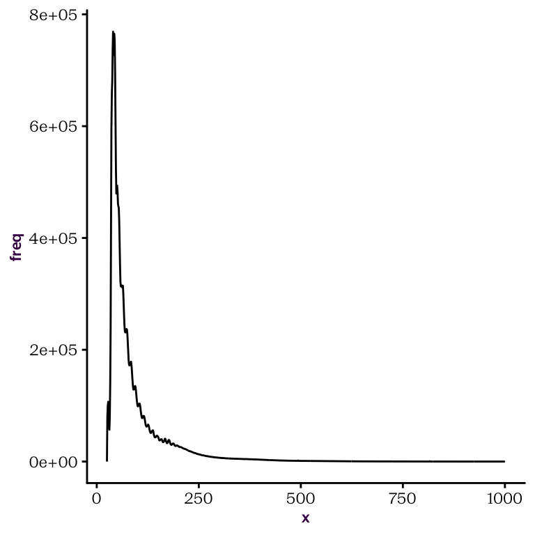
Figure 22.1: Default plot() call on dist with l type produces a line plot, or frequency against size.

Exercise 22.4 Calculate the peaks from 0 - 120 bp.

Exercise 22.5 Define a new custom function (myPlot()) that takes three arguments (1 essential, and 2 optional): x, xRange = c(0,1000), lines = NULL. Your function should do three things:

1. Filter x according to the provided xRange. We will use dist for x when we call the function.
2. Plot x according to the plot type specified in type (e.g. “peaks”, “troughs”).
3. Add vertical lines and labels for their positions if a vector is provided under the lines argument.

Once you have established your custom function. You should be able to produce the following plots.

myPlot(dist, c(50, 150))

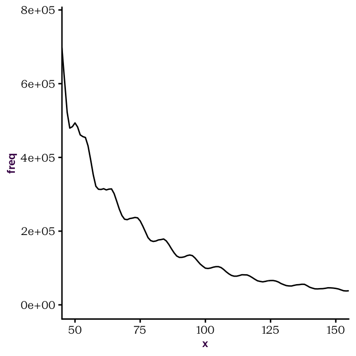
Figure 22.2: Identify peaks and troughs.

myPlot(dist, c(50, 150), "peaks")

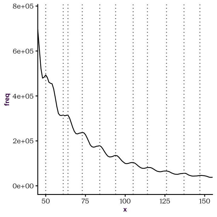
Figure 22.3: Identify peaks and troughs.

myPlot(dist, c(50, 150), "troughs")

Figure 22.4: Identify peaks and troughs.