Chapter 19 Case Study: TaqMan Analysis
19.1 Learning Objectives
By the end of this chapter you should be able to:
- Use
dplyrto apply transformation and aggregation functions
For the extra case studies please see the extra repository here.
Quantitative55 Real-time PCR (qRT-PCR, or simply qPCR) is a popular method to perform relative or absolute quantification of specific mRNA or DNA species (i.e. probes/sequences). There are many techniques popularly used. In this case study, we’ll focus on Taq-Man, a system provided by Applied Biosystems.
In this system, fluorescence of a probe increases each round of a PCR reaction. During the exponential phase, the point at which the fluorescence signal surpasses the background noise is called the threshold cycle (\(C_t\)). The smaller the \(C_t\) is, the higher the initial concentration is (it can reach the exponential phase sooner).
The difference between the \(C_t\) of an experimental probe and an endogenous control (e.g. Gapdh or, in this case, 18S-RNA) conducted on the same sample determines the relative abundance of a sequence/probe (i.e. the \(\Delta{}C_t\)). The \(\Delta{}C_t\) of an experimental sample is then further compared to a control sample to produce the \(\Delta{}\Delta{}C_t\). Finally, to get fold-change of the experimental sample compared to the control sample, we calculate \(2^{-\Delta{}\Delta{}C_t}\).
Each reaction is calculated in triplicate, on a 96 well plate. These triplicates need to be first aggregated. In addition, there can be many probes on a single plate. We’d like to develop a script that can handle any plate, independent of the number of names of the probes used. The out-put from the initial analysis is either an excel file or a flat tab-delimited file (.txt).
19.2 Import the data
The first challenge is to import the data. You have been provided with two files: Atrogin1.txt and MyoD1.txt. We’ll use Atrogin1.txt to develop our script and see if we can make it generic enough to handle MyoD1.txt as well.
Atrogin1.txt. Make sure to check the structure of the file and consider which arguments you’ll need to use to read in a properly formatted data set! Save your data set as qPCR.
Convert qPCR to a tibble and examine it’s structure with glimpse().
To help us make sense of this data, figure offers to visualisations, both depicting the \(\Delta{}C_t\), which we will calculate below. On the left, we see that we have:
- 9 samples, each having 4 – 5 individual technical replicates
- 3 probes, Atrogin 1, HDAC 4, and MURF1
- 2 treatments c and d
- 2 genotypes -/- (knock-out) and +/+ (wild-type)
On the right, we can see that comparing \(\Delta{}C_t\) values between different treatments already shows that there is going to be some interesting results.
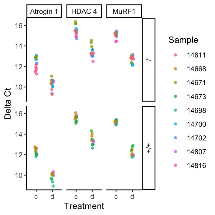
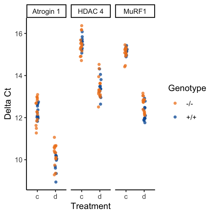
Figure 19.1: Summary visualisations of the data in Atrogin1.txt
19.3 Clean up the data
In this section will build a long sequence of dplyr commands to clean up the data set. For each exercise add onto the previous piece using the \%>\% operator.
c or d.
Exercise 19.4 (2) Select only the variables of interest:
- Well
- Sample
- Detector
- Ct
Exercise 19.5 (3)
The sample variable actually contains three variables. Split it up into three columns, called:
- Treatment
- Genotype
- Sample
Exercise 19.6 (4) Cluster the data into groups according to all four of the following variables:
- Well
- Treatment
- Genotype
- Sample
Here, it’s important to group according to Well since each well contains two probes, the endogenous control and the experimental. This will allows us to select value pairs that we know belong together. That’s very important!
Exercise 19.7 (5)
Since we’re going to perform transformation functions between the EC and the Ct, we’re going to separate the data in a way that allows this to be easy for us. We could have used spread(), but since we have two different detectors and a common Endogenous Control, we have to be a bit more flexible. For each of the groups defined above, calculate the following variables.
- EC The Ct of the Endogenous Control, i.e. the value of the
Ctvariable where theDetectorequals18S rRNA. - Ct The Ct of the Experimental probe, i.e. the value of the
Ctvariable where theDetectorDOES NOT equal18S rRNA. - Detector The name of the detector in the
Detectorvariable that DOES NOT equal18S rRNA.
Finally, save the data set as itself, qPCR. When you glimpse() your data set, it should look like this:
# Observations: 162
# Variables: 7
# Groups: Well, Treatment, Genotype [162]
# $ Well      <int> 56, 57, 58, 59, 60, 61, 62, 63, 64, 65, 66, 67,…
# $ Treatment <chr> "c", "c", "c", "d", "d", "d", "c", "c", "c", "d…
# $ Genotype  <chr> "-/-", "-/-", "-/-", "-/-", "-/-", "-/-", "-/-"…
# $ Sample    <chr> "14611", "14611", "14611", "14611", "14611", "1…
# $ EC        <dbl> 11, 12, 11, 12, 12, 12, 12, 12, 12, 12, 12, 12,…
# $ Ct        <dbl> 23, 23, 23, 22, 22, 22, 25, 25, 25, 22, 22, 22,…
# $ Detector  <fct> Atrogin 1, Atrogin 1, Atrogin 1, Atrogin 1, Atr…
19.4 Calculate summary statistics
We need to also calculate the aggregated data to get the actual \(\Delta{}C_t\) values. Again, begin with qPCR.
Exercise 19.8 (6) Cluster the data into groups according to all four of the following variables:
TreatmentGenotypeDetector
Exercise 19.9 (7)
Calculate the average (avg) and the SEM (SEM) of each technical triplicate for both the Ct and EC variables.
Exercise 19.10 (8)
Apply a transformation function to calculate:
- DeltaCt,
Ct\_avg - EC\_avg
Exercise 19.11 (9)
Ungroup the data frame and regroup according to Detector.
Exercise 19.12 (10) Apply a transformation function to calculate:
- DeltaDeltaCt
DeltaCt - DeltaCt[Genotype == "-/-" \& Treatment == "c"] - FC
2\^{}-(DeltaDeltaCt) - MaxFoldChange
2\^{}-(DeltaDeltaCt - Ct\_SEM) - MinFoldChange
2\^{}-(DeltaDeltaCt + Ct\_SEM))
Save your resulting data frame as itself. The fold-change values are depicted in figure 19.2. Check to see if the values you calculated match what is reported there. The data frame should look like this:
# Observations: 12
# Variables: 12
# Groups: Detector [3]
# $ Treatment     <chr> "c", "c", "c", "c", "c", "c", "d", "d", "d"…
# $ Genotype      <chr> "-/-", "-/-", "-/-", "+/+", "+/+", "+/+", "…
# $ Detector      <fct> Atrogin 1, HDAC 4, MuRF1, Atrogin 1, HDAC 4…
# $ EC_avg        <dbl> 12, 12, 12, 12, 12, 12, 12, 12, 12, 12, 12,…
# $ Ct_avg        <dbl> 24, 27, 27, 24, 28, 27, 22, 25, 24, 21, 25,…
# $ EC_SEM        <dbl> 0.074, 0.087, 0.123, 0.113, 0.124, 0.071, 0…
# $ Ct_SEM        <dbl> 0.205, 0.177, 0.137, 0.133, 0.137, 0.085, 0…
# $ DeltaCt       <dbl> 12.3, 15.5, 15.1, 12.3, 15.5, 15.2, 10.3, 1…
# $ DeltaDeltaCt  <dbl> 0.000, 0.000, 0.000, -0.073, 0.069, 0.089, …
# $ FC            <dbl> 1.00, 1.00, 1.00, 1.05, 0.95, 0.94, 4.21, 4…
# $ MaxFoldChange <dbl> 1.2, 1.1, 1.1, 1.2, 1.0, 1.0, 4.9, 4.6, 6.0…
# $ MinFoldChange <dbl> 0.87, 0.88, 0.91, 0.96, 0.87, 0.89, 3.66, 3…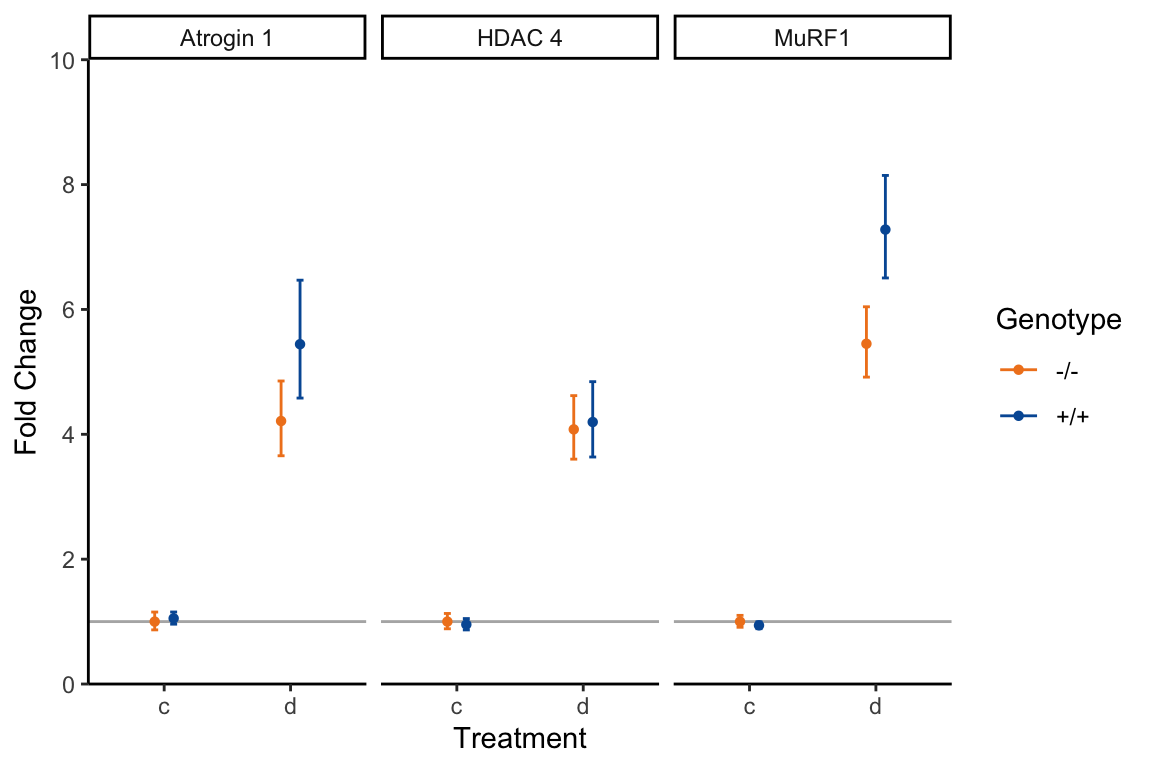
Figure 19.2: Fold change calculations from the Atrogin1.txt file.
19.5 Iterate your Script
Exercise 19.13 (11)
Take the cumulative dplyr commands you’ve written to calculate the fold-change, including importing in the file, and generalise it to use the MyoD1.txt file. The result is depicted in figure .
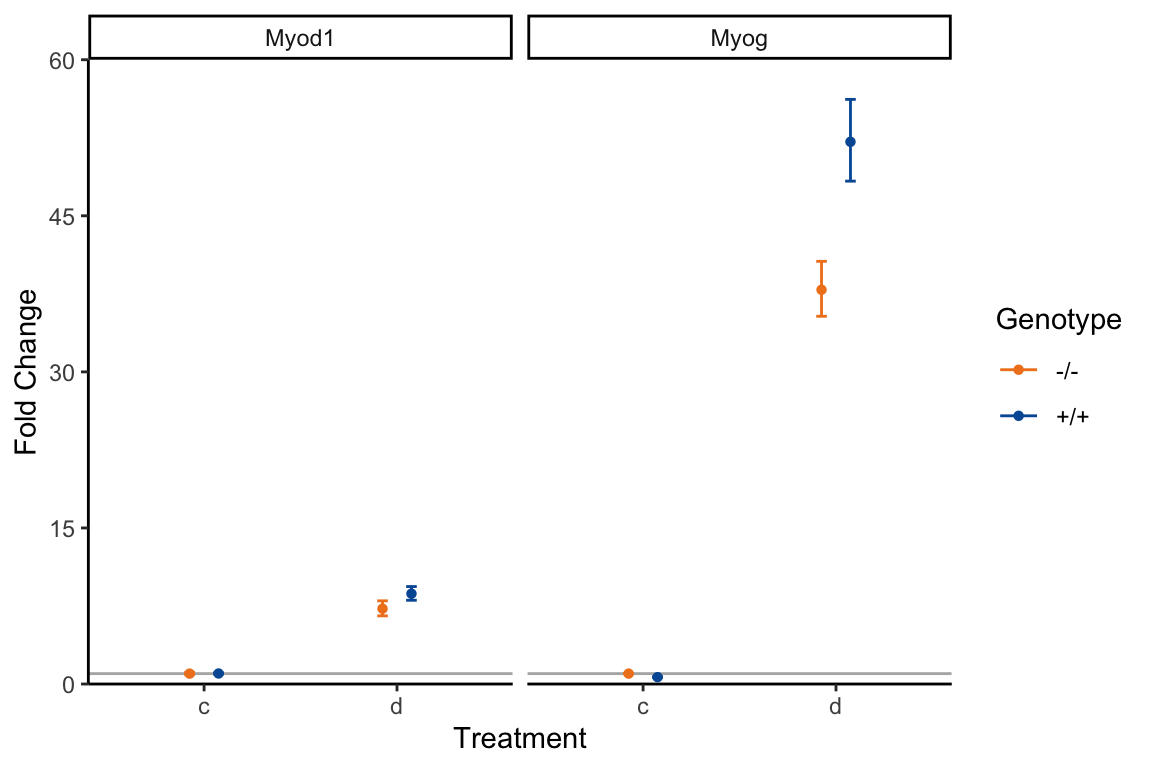
Figure 19.3: Fold change calculations from the MyoD1.txt file.
19.6 Inferential statistics: two-way ANOVA
Let’s move onto the statistics. As above, begin with qPCR and build a complete dplyr command with the \%>\% operator.
Exercise 19.14 (12)
The first five commands (group\_by(), summarise\_at(), mutate(), ungroup(), and group\_by()) are as per the above section, with the exception that here, we’ll group according to four variables:
DetectorTreatmentGenotypeSample
Exercise 19.15 (13)
Calculate a linear model for each detector according to the formula DeltaCt ~ (Treatment + Genotype)\^{2}. Don’t forget to specify the data argument in lm(), since this is not a dplyr function and it is not the first argument – use the . notation for this. Progress to calculate an ANOVA table from the linear models and reiterate this over all the groups.
Exercise 19.16 (15) Extract only the following columns of interest:
Detectortermp.value
# # A tibble: 12 x 3
# # Groups:   Detector [3]
#    Detector  term                 p.value
#    <fct>     <chr>                  <dbl>
#  1 Atrogin 1 Treatment           4.92e- 8
#  2 Atrogin 1 Genotype            3.12e- 1
#  3 Atrogin 1 Treatment:Genotype  4.93e- 1
#  4 Atrogin 1 Residuals          NA
#  5 HDAC 4    Treatment           3.18e- 8
#  6 HDAC 4    Genotype            9.43e- 1
#  7 HDAC 4    Treatment:Genotype  7.78e- 1
#  8 HDAC 4    Residuals          NA
#  9 MuRF1     Treatment           3.79e-13
# 10 MuRF1     Genotype            1.41e- 1
# # … with 2 more rows
qRT-PCR, not to be confused with RT-PCR (reverse transcription PCR).↩