Chapter 3 Getting Started

3.1 Learning Objectives

Begin understanding R’s three key strengths:

Data manipulation (aka data munging),
Statistical modelling, and
Data visualisation.

3.2 Introduction

In this section, we’ll introduce some R fundamentals:

The RStudio IDE,
Keyboard shortcuts,
Basic R notation,
R help pages,

We’ll wrap up by going through a complete and simple data analysis workflow using some advanced functions and concepts, such as the tidyverse package and performing statistics.

Don’t worry if you don’t understand everything! This section will introduce you to thinking about your data in a programmatic way. We’ll return to all these concepts in more depth throughout the workshop and you’ll apply them to your own data.

3.3 RStudio

RStudio is an Integrated Development Environment (IDE). This means that it’s an interface to R, which is installed separately on your computer, it is not R itself. IDEs still use keyboard-entered commands, but they provide several advantages, including:

An integrated text editor with syntax highlighting,
Object viewer (e.g. data frames),
Integrated help pages and graphics device,
Tab auto-complete,
Keyboard shortcuts,
Templates for various output formats, and
Separate projects.

Let’s take a look at projects. This is an an excellent way to separate all the different data analysis scripts into discrete environemts.

Exercise 3.1 (Setting up your project) - Open RStudio and select File > New Project \dots. Alternatively, you can use the projects pull-down menu in the upper-right corner.

Choose Version Control and then Git in the next window.
In the final window, enter the repository URL https://github.com/Scavetta/DAwR. If you press tab the name field will automatically fill in, if not just call it DAwR. In the third field, use the browse button to choose a convenient destination for your projects. I have mine in ~/Documents/R Projects. You don’t need to open this in a new session, so leave the checkbox unchecked.

RStudio will now download the workshop files from the GitHub repository. Afterwards, it should state “DAwR” in the upper-right corner.

The RStudio interface will be divided into three panes. You’ll see the fourth pane once you open a new script file in the text editor.

Exercise 3.2 (Starting a script) Use either the file menu or the new document icon to open a new blank R script in the text editor. Alternatively, and preferable, you could type the keyboard shortcut shift + ctrl + n (shift + cmd + n will also work on a Mac).

Make sure the the selector on the lower right corner of the new text document states that it is an . There are many different kinds of scripts that RStudio recognizes.

Always begin every script with a proper header! Type the following into the new file, including the \#, replacing the text inside the <> with the required information:

# <script title>
# <your name>
# <today's date>
# <script description>

Exercise 3.3 (Setting up your project) I also like to begin scripts by removing all objects hanging around from the last session. This doesn't solve all our reproducibility problems, but it’s a good start for when we have a fresh session.

Type the following into the new file. We're not actually executing any code here, we’re just setting things up.

# Clear workspace:
rm(list = ls())

Exercise 3.4 (Load packages) It’s also good style to list the packages you'll use in your project at the beginning of your main script. Type the following into the new file:

# load packages:
library(tidyverse)

Now that we have the start to our script set up, let’s look at what’s in the four panes:

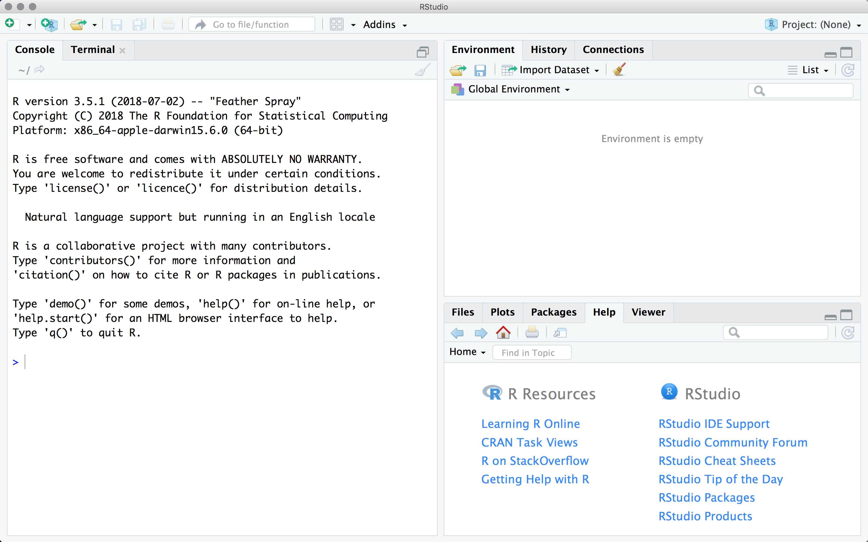The RStudio interface showing the help pane in the lower right.

Upper-left is the text editor and object viewer. Adding a new R script will open a second tab in this pane, like a web-browser.

Upper-right lists all the objects we have defined, and also provides access to our command history.

Lower-left is the R console. This is where R actually lives - all the commands will be executed here. If you don’t see it here, it wasn’t executed.

Lower-right has tabs for files in our working directory, all the plots we have made in this session, a listing of all available packages, and easy access to the help pages.

In fig. Rstudio, the result of the example from this chapter is shown. The PlantGrowth data-set is shown in the upper-left pane. In the lower-left pane, the commands for drawing the box plot and calculating the mean of each condition have been executed. The two panes on the right show the results. In the upper-right pane, the m object, containing the mean values of each group is visible, in addition to the previously defined linear model and ANOVA results. In the lower-right pane, the resultant box-plot is presented.

3.4 The R Console

The standard R installation provides users with a simple console. Individual commands are written at the prompt and executed by pressing the Enter key. You can do the same directly in the console in RStudio.

3.5 The Text Editor & R Syntax

RStudio’s built-in text editor offers a more flexible and convenient way of managing commands. Execute commands from the text editor by using the keyboard shortcut ctrl + Enter (or command + Enter on a Mac).²

For single and multi-line commands, you don’t need to highlight the command or even have the cursor at the end of the line. So don’t waste time fiddling with your mouse! The entire command will be excuted, regardless of where the cursor is positioned. If you do highlight only a portion of a long command, only that segment will be executed. That’s pretty useful for finding errors in long commands.

In this book, R input and output is presented in mono-spaced font, as shown below.

Exercise 3.5 (R Syntax) Can you guess what the following commands will do? Type then into your text editor and execute them to find out.

# R syntax
n <- log2(8) #The logarithm of 8 to base 2
n

The above command computed \(log_{2}\left(8\right)\) and assigned the result to the object n, which it created on-the-fly. The result is associated with an index position. In this case, there is only one answer (3), and it is at position 1. {#logExample}

The following table will help you to make sense of the above example.

Table 3.1: R’s syntax.
Notation	Description
`>`	The R command prompt.
`n`	An object name.
`<-`	The assign operator.
`log2()`	The function to be solved. The solution will be assigned to n.
`8`	The function’s argument.
`#`	The beginning of the comment.
`The logarithm of ...`	The comment.
`[]`	Refers to the index of the output.
`1`	The index number.
`3`	The value at position `[1]`.

Exercise 3.6 (Incomplete commands) So far, so good. But what would happen if you executed the following command? Do you think it will result in an error?

n <- log2(8

The above command doesn’t result in an error because it’s not an incorrect command, it’s an incomplete command. If an incomplete command is executed the > prompt in the console will turn into a + sign to indicate that further information is needed. In this case, it’s better to just go in the console and press the ESC key, correct the command and then reexecute it. Make sure you remove the above incomplete command from your script or you’ll run into problems eventually.

3.6 The Assign Operator: Creating Objects

We’ve already encountered our first object (n), operator (<-), function (log2()) and argument (8). We’ll keep returning back to these concepts throughout the workshop.

We used the assign operator, <- to assign a value to an object. You can enter <- using the keyboard short cut Alt + - (also Option + - on a Mac).

Although it is possible, and you will inevitably encounter it, I recommend to never use = as the assign operator. It can lead to confusion, especially for beginners, and is therefore typically considered bad style.⁴

Just for convenience, I’ll use some very simple, one-letter names for objects. However, in practice you’ll find it very useful to name objects in a meaningful way. Do not use names of pre-existing functions, like data or subset or plot!

Assigning a result to an object does not typically produce any output. If we want to see the contents of an object, we can look in RStudio’s environment pane, or, as we did above, just execute the name of the object, n in the console. When we execute an object name in the console, it’s actually a short cut for:

print(n)

R looks at the class of the object and decides what’s the best way to print it to the screen. We’ll return to classes in a later section.

3.7 R Help Pages: Functions

It’s worthwhile familiarizing yourself with R’s help pages. To get the most out of the help pages, you will need to understand what functions and packages are. Functions will be discussed in detail in section 6. However, the help pages will make more sense when you know the following simple definitions.

Functions are commands that take on specific arguments. In this text, functions are written in mono-spaced font followed by brackets: name().
Packages are collections of functions.

The easiest way to get help on a function is to type its name into the search box in the help pages. Some other useful commands are:

Table 3.2: Accessing R’s help pages for specific functions and topics.
Command	Outcome
`help(topic)`, `?topic()` or `?topic`	Calls the `topic()` function help page.
`help.search("topic")` or `??topic`	Searches all help pages for the word “topic”. This is useful if you’re not sure what function to use.
`example(topic)`	Executes all the commands contained in the examples sub-section of the `topic()` help page.

For example, the command log opens a help page, with details on how to use the log() function, titled Logarithms and Exponentials⁵

Exercise 3.7 (R Syntax) Using the commands in table 3.2, search for the R function that calculates the standard deviation. Notice that when you run the example, the command prompt changes.

Familiarize yourself with the different sections of the help page for the function that calculates the standard deviation. Use table to find the command to run the example at the bottom of the help page directly in the R console. You should not have to type or copy the example.

Table 3.3: The anatomy of a help page in R. Other sections may be added by the help page’s author. They are typically self explanatory.
Section	Description
`Description`	A description of what the function does in simple language.
`Usage`	An example of how the function is used, showing all its essential and optional arguments.
`Arguments`	A description of the arguments available, plus the specific data types and structures they accept.
`Details`	Points of caution and interest to watch out for.
`Value`	The output returned by the function.
`References`	Publications which describe the function. Particularly useful for modern methods in statistics.
`See Also`	Recommendation for similar functions that may be more appropriate for the tast at hand.
`Examples`	Reproducible example code that demonstrates how to use the function.

For optional arguments, their default values are given. If no default value is given, the argument is essential and it must be provided when called.

3.8 Packages: Extending R’s Functionality

The core R installation is called the base package. This is actually a collection of several packages, each of which has a collection of functions. For example, in your initial installation you’ll have the utils (i.e. utilities), graphics (for basic plotting), and stats (for basic statistics) packages. In addition to this, there are over 12,500 packages in the official repository, CRAN (the comprehensive R archive network) and over 1,500 Bioinformatics-focused packages in the BioConductor repository. On top of all that there are thousands more published on GitHub, an online repository for code of all varieties, and many ore in-house packages not released to the public. All these packages act as functional add-ons to the base package, kind of like extensions in your web-browser. You can install packages directly from CRAN using RStudio’s packages pane. BioConductor and GitHub packages are beyond the scope of this workshop. Table @ref{tab:help-pack} lists the most common functions for working with packages.

Table 3.4: Help using packages. Replace `name` with the specific package name you are interested in.
Command	Outcome
`install.packages(name)`	Install package `name`.
`library(name)` or	Initialize package `name`.
`library()`	List all installed packages.
`library(help = name)`	Provides details, including all functions, contained in `name`.
`search()`	List the search space.

Always install all dependencies when you install a package. Installation can also be done through the R console menu. A package only needs to be installed once, but must be initialized every time you start a new R session. After initialization, you will have access to all the functions within that package. You can access a specific function within a package, without explicitly loading the package, by using the double colon operator, ::.

We’ll use the tidyverse package throughout this workshop. It’s actually a suite of packages. All packages can be considered as a collection of packages because they all have dependencies on other packages. When you install one, you’ll also be installing all the other packages that it depends on.

Exercise 3.8 (Install the tidyverse packages) Install the tidyverse package by using the packages panel in the lower-right pane. Make sure you are installing from the CRAN repository and that the “Install dependencies” option is selected.

Table 3.5: Packages in the `tidyverse`.
Package	Uses
`dplyr`	A grammar of data manipulation.
`readr`	Simplify the import of rectangular data (txt, csv).
`tibble`	A modern version of the data frame.
`stringr`	Simplifies working on strings (characters).
`tidyr`	Create tidy data.
`forcats`	Simplifies working with categorical data.
`purrr`	A toolkit for reiterating functions on elements of various data types.
`lubridate`	Simplifies working with dates and times.
`ggplot`	Create elegant data visualizations.

Exercise 3.9 (R Syntax) Now that we’ve installed the the suite of packages, we can execute it.

You only have to install the package once, but it must be initialized each time we start a new R session. Remember that we typed the following command at the top of our script?

library(tidyverse)

You can also use ctrl + R (or command + R on a Mac), or use the icons to run the line of code where the cursor is positioned.↩
Use ↑ and ↓ at the command prompt to scroll through the history of entered commands.↩
There is a third option, ->, which we’ll encounter in section @ref(dplyr_arrange)↩
Replace topic with the specific function or search term you need help with.↩