Chapter 16 Case Study: Effects of Meditation
To understand the usefulness of tidy data and dplyr, consider the meditation data-set. This data-set contains the expression values of 6 pro-inflammatory genes. The researchers wanted to test if these genes are differentially expressed after meditation in people who regularly meditate, compared to non-meditating control individuals. Expression levels were measured in the morning (time 1) and after (time 2) a full day of meditation, by experienced meditators, or leisure, by the control group.
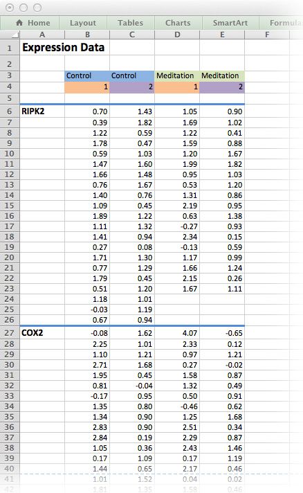
Figure 16.1: The medi data-set as it would be typically stored as an Excel spreadsheet. Although this is human-readable, it is not an efficient way of storing data!
Figure 16.1 is an example of a typical Excel spreadsheet. Here, column headers are found in the middle of the spread sheet and the results for each measured gene is contained in its own table on the same worksheet. In addition, column headers are colour-coded and there is plenty of white space for formatting purposes.
As a first step towards tidy data, we will remove all white space, colour-coding and floating labels. The data-set in Figure 16.2 resembles the long list file we have already encountered. It’s not perfect, but it’s a good start for working with R.
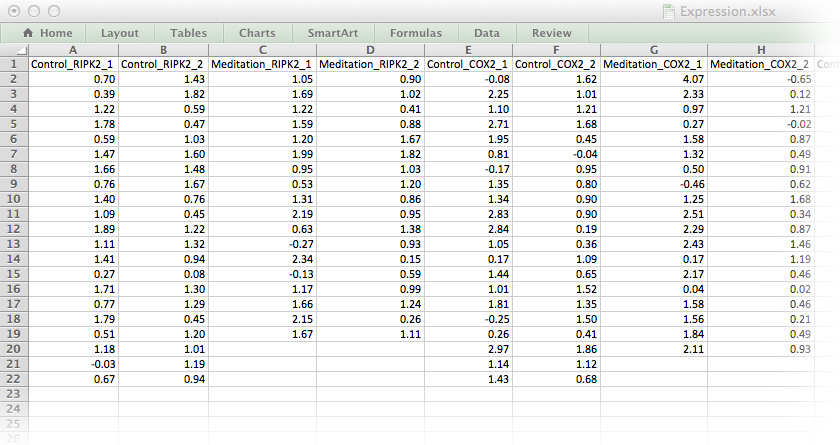
Figure 16.2: The medi data-set in a format ready for importing into R.
Expression.txt. Save it as an object called medi and convert it to a tibble.
Confirm that medi has the dimensions 21 x 24.
gather(), it tries to guess which variables are the best choice. To do this, gather() uses categorical variables and then any column headers of continuous data as ID variables. However, recall that the medi data-set doesn’t have any categorical variables, so in this case gather() will take all our column headers as a single ID variable.
gather(): key and value.
# [1] 21 24# Observations: 504
# Variables: 2
# $ key <chr> "Control_RIPK2_1", "Control_RIPK2_1", "Control_RIPK…
# $ value <dbl> 0.70, 0.39, 1.22, 1.78, 0.59, 1.47, 1.66, 0.76, 1.4…The last action we need to perform before we can start working on this data is to separate the three variables contained in the variable column into distinct columns. For this we will use the tidyr::separate() function. Split up medi.t$key and overwrite medi.t with the new columns and the original values.
medi.t, 504, is the product of the original data-set’s dimensions, 21 and 24.
# Observations: 504
# Variables: 4
# $ treatment <chr> "Control", "Control", "Control", "Control", "Co…
# $ gene      <chr> "RIPK2", "RIPK2", "RIPK2", "RIPK2", "RIPK2", "R…
# $ time      <chr> "1", "1", "1", "1", "1", "1", "1", "1", "1", "1…
# $ value     <dbl> 0.70, 0.39, 1.22, 1.78, 0.59, 1.47, 1.66, 0.76,…
16.1 A Review of the 5 dplyr Verbs
Now that we have tidy data, let’s review some of the functions from the package:
filter subsets the data frame. Alternatively, we could have used the base package function subset() or [].
# [1] 205 4# [1] 168 4# [1] 474 4select chooses specific variables
# [1] "gene"# [1] "treatment" "time" "value"We can also rename variables as we select them:
# Rename variables:
# Remember, select() keeps only the variables specified:
medi.t %>%
  select(expressionValues = value)
# # A tibble: 504 x 1
# expressionValues
# <dbl>
# 1 0.7
# 2 0.39
# 3 1.22
# 4 1.78
# 5 0.59
# 6 1.47
# 7 1.66
# 8 0.76
# 9 1.4
# 10 1.09
# # … with 494 more rows# # A tibble: 504 x 4
# treatment gene time expressionValues
# <chr> <chr> <chr> <dbl>
# 1 Control RIPK2 1 0.7
# 2 Control RIPK2 1 0.39
# 3 Control RIPK2 1 1.22
# 4 Control RIPK2 1 1.78
# 5 Control RIPK2 1 0.59
# 6 Control RIPK2 1 1.47
# 7 Control RIPK2 1 1.66
# 8 Control RIPK2 1 0.76
# 9 Control RIPK2 1 1.4
# 10 Control RIPK2 1 1.09
# # … with 494 more rowsarrange reorders variables, similar to order().
# reorder according to descending value
medi.t %>%
  arrange(desc(value)) -> medi.t2

# ascending order of gene, then time, then treatment
medi.t %>%
  arrange(gene, time, treatment)
# # A tibble: 504 x 4
# treatment gene time value
# <chr> <chr> <chr> <dbl>
# 1 Control CCR7 1 2.89
# 2 Control CCR7 1 1.44
# 3 Control CCR7 1 1.64
# 4 Control CCR7 1 1.91
# 5 Control CCR7 1 1.65
# 6 Control CCR7 1 1.05
# 7 Control CCR7 1 1.24
# 8 Control CCR7 1 0.73
# 9 Control CCR7 1 1.11
# 10 Control CCR7 1 1.45
# # … with 494 more rowsmutate creates new variables that are functions of existing variables
# # A tibble: 504 x 5
#    treatment gene  time  value stdev
#    <chr>     <chr> <chr> <dbl> <dbl>
#  1 Control   RIPK2 1      0.7  0.683
#  2 Control   RIPK2 1      0.39 0.683
#  3 Control   RIPK2 1      1.22 0.683
#  4 Control   RIPK2 1      1.78 0.683
#  5 Control   RIPK2 1      0.59 0.683
#  6 Control   RIPK2 1      1.47 0.683
#  7 Control   RIPK2 1      1.66 0.683
#  8 Control   RIPK2 1      0.76 0.683
#  9 Control   RIPK2 1      1.4  0.683
# 10 Control   RIPK2 1      1.09 0.683
# # … with 494 more rows
Alternatively, we can use transmute() which will drop existing variables:
# # A tibble: 504 x 1
#    stdev
#    <dbl>
#  1 0.683
#  2 0.683
#  3 0.683
#  4 0.683
#  5 0.683
#  6 0.683
#  7 0.683
#  8 0.683
#  9 0.683
# 10 0.683
# # … with 494 more rows
summarise collapses multiple values to a single value, like in ddply()
# # A tibble: 1 x 1
#   average
#     <dbl>
# 1    1.11
16.2 The group_by() Adverb
So far so good, but of course in split-apply-combine, we are interested in working on sub-sets of our data frame. Therefore, in addition to the five nouns, there is one adverb, which modifies how the verb interacts with the noun. This is the important grouping variable:
group_by() defines the factor variables to use for subsequent actions.
# Treatment and time, grouped according to each gene:
medi.t %>%
  group_by(gene)

# Gene and time, grouped according to each treatment:
medi.t %>%
  group_by(treatment)

# Gene and treatment, grouped according to each time:
medi.t %>%
  group_by(time)

# Time, grouped according to each gene and treatment:
medi.t %>%
  group_by(gene, treatment)

# Treatment, grouped according to each gene and time:
medi.t %>%
  group_by(gene, time)

# Genes, grouped according to each treatment and time:
medi.t %>%
  group_by(treatment, time)

# All 24 combinations, grouped according to gene, treatment and time:
medi.t %>%
  group_by(gene, treatment, time)
The grouped by object is still a data frame, but it has a new class attribute associated with it, which tells other dplyr functions how to group sub-sets.
# [1] "grouped_df" "tbl_df" "tbl" "data.frame"Exercise 16.3 (Calculate Statistics) Consider the structure of the data frame below. Using functions calculate each of the following statistics for each of the unique 24 combinations of gene, treatment and time:
averagethe mean of the valuenthe number of observations in each groupSEMThe standard error of the meanCIerrorThe 95% CI error defined by the t distributionlower95The upper 95% CI limitupper95The upper 95% CI limit
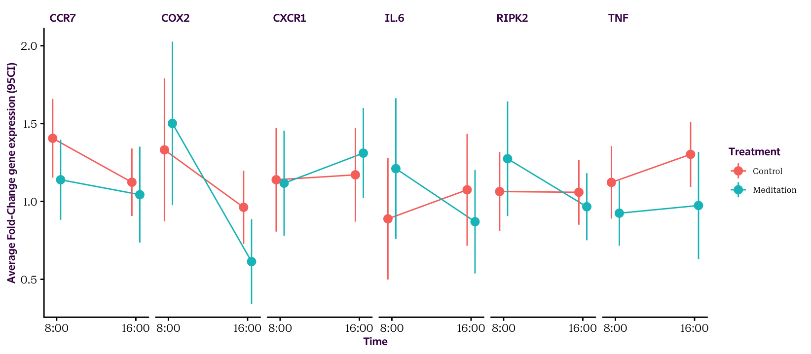
Figure 16.3: Gene expression averages and 95 CIs.
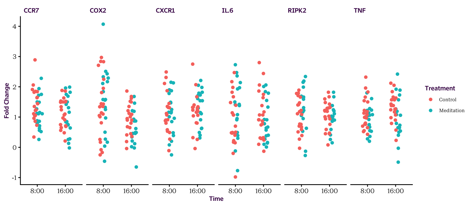
Figure 16.4: The raw values.
Exercise 16.4 (Export data) Now that you've processed your data, refer back to the chapter on importing data and see if you can get a file on your computer that contains the summary statistics. See section @(exporting).
Exercise 16.5 (Calculate ANCOVA)
The broom package contains two functions to make applying statistical tests in a tidy format easy: do() and tidy(). See if you can calculate an ANCOVA for each gene in one command. Remember we saw how to calculate an ANOVA in the first chapter, an ANCOVA is a variant with a continuous predictor variable (here time). Out model will be defined as value ~ treatment + time.
This is the result for only RIPK2:
| Df | Sum Sq | Mean Sq | F value | Pr(>F) | |
|---|---|---|---|---|---|
| treatment | 1 | 0.07 | 0.07 | 0.22 | 0.64 |
| time | 1 | 0.41 | 0.41 | 1.31 | 0.26 |
| Residuals | 75 | 23.38 | 0.31 | NA | NA |
In the end you should have a table that reports all the following values: